Sustainable Places Research Institute, Cardiff University. School of Planning and Geography, Cardiff University. 1. INTRODUCTION. In a world facing both ...
13th Annual Transport Practitioners’ Meeting 2015 – PTRC – London – 1-2 July
3D NETWORK MODELS FOR PREDICTION OF CYCLIST FLOWS Crispin Cooper and Alain Chiaradia Sustainable Places Research Institute, Cardiff University School of Planning and Geography, Cardiff University 1. INTRODUCTION In a world facing both resource depletion and global warming, and in societies facing obesity as well as transport congestion problems, the use of cycling for transportation seems like a good idea. We are not the first to say this! Forsyth et al (2009) documents the promotion of cycling as sustainable transport from the 1960s onwards. There is currently therefore, considerable interest among planners both in catering to the needs of existing cyclists, and in encouraging non-cyclists to switch to this option. There is no simple way to achieve these aims, and in particular the literature suggests that only comprehensive packages of policies can help to achieve the latter (Pucher, Dill, and Handy 2010; McCormack and Shiell 2011; Forsyth and Krizek 2010; 2011; Handy, Wee, and Kroesen 2014). For better or worse, the benefits of active travel schemes are principally evaluated on a financial basis; the primary benefit from this perspective is usually the saving to healthcare providers dealing with a more active population, although a secondary saving arises from increased safety of those who are already active (sample analyses of this type include Wilson and Cope 2011; Canning, Millar, and Moore 2012). Various authors, possibly inspired by the overlap of cycling with public health issues, have noted the need for developing a more robust quantitative evidence base for cycling in urban planning (Krizek, Handy, and Forsyth 2009), more reliable and better validated GIS measures, e.g. for street patterns (Brownson et al. 2009) and better ways to ensure integration of new infrastructure with the “continuous network” (Forsyth and Krizek 2011). Traditional transport modelling methods have to date had limited application in the modelling of active travel, due to their focus on large scale transport analysis zones rather than small, link-level features which affect the travel decisions of pedestrians and cyclists (Cervero 2006). This paper therefore focuses on spatial network analysis (SNA), which offers an alternative to traditional methods for predicting fine-grained flows on networks, by working at network link level. Karou and Hull (2014) demonstrate the use of SNA to measure accessibility to public transport, and Zhang et al (2015) show a strong link between various network centrality measures and accidents involving nonmotorists. Returning to the prediction of flows, Lowry (2014) uses SNA to interpolate from a small set of measured vehicle flows to the remainder of the road network, using shortest path betweenness. In the case of bicycles, spatially localized angular betweenness (reviewed in Cooper 2015) is used in a series of space syntax studies (Raford, Chiaradia, and Gil 2007; Manum and Nordstrom 2013; Law, Sakr, and Martinez 2014), often in combination with other
variables, to predict flows of cyclists on the network. Angular betweenness is a measure which identifies the links most commonly used in straightest-path (rather than shortest-path) routes through the network. While this does correlate with flows of cyclists to some extent, angular betweenness is the exact same measure used in the space syntax tradition to predict flows of vehicles and pedestrians (Hillier and Iida 2005). Combining angular betweenness with other factors in a multivariate regression model could thus be viewed as postprocessing (Cervero 2006) a single underlying direct demand transport model which - apart from the straightest-path aspect - is similar to Lowry’s (2014) vehicle model. Prior to post-processing, such a model differentiates between the navigational choices of drivers, cyclists and pedestrians only in terms of the distance that each are willing to travel. Common sense suggests that these three classes of road user are in fact likely to choose routes in a different manner; the observation of Raford et al (2007) that preferred cyclist routes are often parallel to, but not coincident with routes of high angular betweenness would also suggest this possibility, and discrete choice modelling in fact confirms it (Broach, Dill, and Gliebe 2012; Wardman, Tight, and Page 2007). Related to the problem of predicting bicycle flows, is the problem of predicting trip generation, trip distribution and mode choice, i.e. whether or not people will travel in the first place, where they will choose to travel and whether they will choose to cycle. For the purpose of this paper we group these three phenomena into a single model of cycle trip demand. Any model of cycle flow must contain at least some assumptions on trip demand, if not an explicit model. For the environmental, social and economic policy reasons noted above, the question of whether and to what extent new infrastructure affects the number of people who choose to cycle is an area of active research. Note however, that a model of cycle demand for individual trips is not necessarily the same as a model of cycle demand for the aggregate population. Feedback loops such as the land use-accessibility cycle (Chiaradia, Cooper, and Wedderburn 2014 contains a brief review), and residential self-selection (Cervero 2006) will mean that keen cyclists may deliberately choose to live near a suitable route for cycling to work, or perhaps that an abundance of opportunities for cycling will lead to a population more willing to consider cycling as a mode of transport. Thus, in addition to models of mode choice for individual routes (e.g. Wardman, Tight, and Page 2007) there exist numerous models of mode choice at district level, which aside from being necessary, are advantageous to explore due to the better availability of data at this level. Some of these models have been unable to discern any effect of infrastructure on cycling (Pooley et al. 2011; Goodman et al. 2014) while others have (Winters et al. 2013; Ewing et al. 2014; Parkin, Wardman, and Page 2007; the latter being endorsed by Department for Transport 2014b). Parkin et al (2007) find a strong correlation between the proportion of off-road cycle route at local authority level, and decision to cycle to work at ward level; however this model does not account for the location of off-road route, and so from the perspective of urban design is not sensitive to the location options a planner might consider. There is also little history of any such district level models being used to predict cycle flows at network link level; traditionally, cycle mode choice and hence demand is considered exogenous to existing transport models such as TRIPS and QUOVARDIS (Schwartz et al. 1999) which themselves tend to operate on a simplified network suitable for motor vehicles rather than cyclists.
13th Annual Transport Practitioners’ Meeting 2015 – PTRC – London – 1-2 July 3D Network Models For Prediction Of Cyclist Flows | Crispin Cooper, Alain Chiaradia
2
The contribution of the current study is to provide a nuanced model of cycle flow, using spatial network analysis on a detailed network, that is sensitive to both to infrastructure changes and to the differences in behaviour of cyclists and car drivers, and is hence of increased use in planning decisions. As it handles route finding decisions of drivers and cyclists separately, the model presented is also applicable to road safety models examining the interaction between the two classes of road user. We conclude by discussing avenues for modelling the effect of infrastructure on demand for cycling. The model is based on discrete choice literature which studies the effect of distance, turns, slope and vehicle traffic on cyclist route choice, combined with the SNA tradition of spatially localized betweenness reviewed in Cooper (2015). It will be shown that this is equivalent to a mode choice model which accounts for the effect of urban density on the decision to cycle. The approach can perhaps be classed as ‘extreme’ spatial network analysis in that it considers network accessibility itself to be the primary driving cause of land use and hence trip generation, resulting in a model which is low cost with respect to data collection requirements: at a minimum the model can function using only the network itself as input, although in the current case we calibrate using measured flows. The model is reproducible using publicly available, general purpose network analysis software sDNA+, which can function either as a GIS or CAD plugin (Chiaradia, Cooper, and Webster 2011). 2. METHODS 2.1.
DATA
Our spatial network is based on Open Street Map (OSM). OSM is an open access, crowd sourced mapping product with global scope; while coverage is currently patchy, both coverage and data quality are only likely to increase for the foreseeable future, and for coverage of cycle routes OSM is currently the best on offer in the UK (Lovelace 2015). The OSM network is however, still liable to contain spatial errors which are detected and repaired as described in Cooper (2014a; 2014b). Figure 1 shows a map of all cycle sampling locations and counts used in the study. Two sources of cycle flow data were used to calibrate the model: 1. Department for Transport (DfT) (2014a) pedal cycle flows, which are derived from a mixture of vehicle gates and manual sampling at 107 locations in Cardiff. The DfT report annual average daily traffic (AADT). However, only locations on roads carrying vehicle traffic are recorded, so this data gives no indication of the use of traffic free routes. The DfT deem any weekday from March-October to be a ‘neutral day’ on which a representative sample of traffic can be taken; AADT is estimated by applying expansion factors based on type of road, day of year and type of vehicle. Thus while this methodology takes account of national weather variations it discards regional ones, which may have a major effect on pedal cycle usage. Additionally, it may underestimate recreational pedal cycle traffic on weekends. Finally, in some cases roads are not sampled at all, but flows are estimated by applying a
13th Annual Transport Practitioners’ Meeting 2015 – PTRC – London – 1-2 July 3D Network Models For Prediction Of Cyclist Flows | Crispin Cooper, Alain Chiaradia
3
growth factor to count data from a previous year (Department for Transport 2011). 2. Cardiff Council’s data, collected from 14 electronic cycle counters on traffic free routes over a 3 month period. Cardiff council report only daily flows for the recorded months (September-November 2014). As cycle traffic is heavily seasonal, a seasonal correction was derived from a 15 th electronic cycle counter which records year round flows, to estimate AADT.
Figure 1 Measured cycle flows in Cardiff. DfT and Council figures both estimate AADT but are not necessarily comparable.
As the two sources of data were collected using different methodologies, we cannot be sure whether or not the AADT flows derived from each are truly comparable (a more detailed discussion of issues with cycle count data can be found in Gordon 2014). However, as both data types are essential to understanding flows of pedal cycles, we must combine them nonetheless. To account for errors generated by the mismatch of methodologies, some of the regression models which follow include a dummy variable to account for the data source. The vehicle flow sub-model is calibrated using vehicle counts from the same 107 locations sampled by the DfT (2014a). Mode choice data is derived from the UK Census (Office for National Statistics 2011) aggregated to output area level, at which there are 1076 zones within the city of Cardiff.
13th Annual Transport Practitioners’ Meeting 2015 – PTRC – London – 1-2 July 3D Network Models For Prediction Of Cyclist Flows | Crispin Cooper, Alain Chiaradia
4
2.2.
TRIP GENERATION, DISTRIBUTION AND MODE CHOICE MODELS
The SNA models of vehicle, pedestrian and cyclist flow cited in the introduction have all used some form of spatially localized betweenness (Cooper 2015) as a predictor of actual flow. In rough terms, this equates to a simulation of indiscriminate trips from everywhere to everywhere, subject only to a maximum trip distance or radius. Although such models are known to fit the data well, it is prudent to consider why this is the case in order to understand the limits of SNA models. Briefly reviewing the mode choice literature, we note the importance of urban density as a common theme among all models which find a link between the built environment and decision to cycle. Winters et al. (2013) considers the effect of bike routes on mode choice, though this is tested only in a univariate model and it is unclear to what extent urban density confounds this relationship. Ewing et al (2014) show a weak relationship between cycle mode choice and several variables (intersection density and connectivity, population and jobs) all of which strongly correlate with urban density. Parkin et al (2007) describe a combined built environment and demographic model which explains a large proportion of variance in cycle use for the journey to work (r2=0.82); in this case the two largest built environment coefficients relate to the proportion of off-road cycle route, and distance travelled. Note that the latter variable will again, on average, tend to correlate with urban density as the existence of numerous job opportunities nearby increases the likelihood that a randomly selected individual will both occupy such a job, and cycle to it. Similar logic also applies both to discretionary and recreational trips. It is thus reasonable to assume that cycle trips correlate with urban density. Following Chiaradia et al. (2014) we take urban density to be defined by the number of network links within a given radius, therefore we choose to weight our simulated trips “from everywhere to everywhere” by network links, i.e. we simulate trips “from every link to every other link”. Thus it is assumed that in the long run, that the spatial network generates accessibility; that accessibility influences land use and hence opportunities and that opportunities generate traffic. The advantage of this is that that feedback cycles such as land useaccessibility and residential self-selection are included in the model without requiring expensive data collection. While we present this as a spatial network model, it can also be characterized as a direct demand transport model in which trip generation, distribution and mode choice are considered congruent (Cervero 2006; Lowry 2014; and Ortúzar and Willumsen 2011, chapter 6). Compared to a traditional transport model, the disadvantage is that the lack of individually calibrated stages means we cannot verify each stage of trip generation, distribution, mode choice and route choice individually. In mitigation of this problem, we explicitly test the link between urban density and mode choice. Returning to SNA terminology, the implication of this demand model is that we compute link weighted betweenness, spatially localized within a Euclidean buffer. The only parameter used to calibrate the model is the radius for network analysis which can be interpreted as a maximum trip distance. This is also how we model competing modes, because at higher radius the incentive is to travel
13th Annual Transport Practitioners’ Meeting 2015 – PTRC – London – 1-2 July 3D Network Models For Prediction Of Cyclist Flows | Crispin Cooper, Alain Chiaradia
5
by motorized transport rather than cycle. Noting that as unimodal approaches to cycle modelling are in widespread use (Department for Transport 2014b) we do not consider any negative effect on cycling of readily available alternatives such as metro transit, in specific locations. 2.3.
ROUTE CHOICE MODEL
The design principle guiding the route choice model is that it should make maximum use of publicly available data to ensure a useful tool is developed for general application. We therefore consider the following four factors: route length, directness, slope and vehicle traffic. The first two of these are derived directly from a spatial network model; the third is obtained by draping the spatial network over a publicly available terrain model such as OS Terrain 50. Vehicle traffic is inferred from an SNA sub-model based only on directness. It is desirable to use actual vehicle flow data to calibrate this model; in the UK this is now freely available (Department for Transport 2014a) and for most planning projects worldwide some degree of existing vehicle flow data is available also. We do not currently consider the effect of on-road cycle lanes as studies on the effectiveness of these show mixed effects, and reliable data on the level of provision is not always available. We do include traffic free cycle routes. To determine the function describing the effect of these four factors (length, directness, slope and vehicle traffic) on cyclist route choice, we take Broach et al. (2012) as a starting point. Broach used a discrete choice model to determine factors affecting cyclists’ choice of routes in Portland, Oregon. Length, traffic and slope are defined as per Broach’s model, though the notion of directness needs modification as Broach only counts turns at junctions on a grid street pattern, not changes of direction along links. We thus take a turn (not across traffic) to equate to a 90° change of direction. We combine these measures through what we have termed a hybrid distance metric for spatial network analysis; the parallel in transport modelling would be a generalized cost expressed in kilometres. This can also be interpreted as a perceived effort, e.g. Broach’s Table 3 implies that a cycle commuter travelling 1km with an upslope of 2-4% perceives an effort equivalent to riding 1.37km. In the case of traffic, we note that most of the vehicle flows in our model fall into the lowest band of Broach’s model. This provides little distinction between levels of vehicle flow, therefore we choose to interpolate between classes of vehicle flow by fitting an exponential curve with a single parameter. We plot each ‘band’ of cost at its lower limit of traffic flow, e.g. the perceived effort of cycling in traffic of 20-30,000 vehicles per day is assumed to apply to 20,000 vehicles per day, as most roads in this each band will have flows close to the lower bound of the band (the distribution of traffic flow over roads tending to exponential tailoff in its upper limits). The exception to this is the 0-10,000 vehicles per day band, for which we take 5,000 vehicles per day to be indicative. For zero vehicles per day we take the perceived effort for a traffic free bike path; 840 metres for a 1km trip. The curve resulting from these assumptions is shown in Figure 2.
13th Annual Transport Practitioners’ Meeting 2015 – PTRC – London – 1-2 July 3D Network Models For Prediction Of Cyclist Flows | Crispin Cooper, Alain Chiaradia
6
Figure 2 Perceived effort for cycling in motor vehicle traffic, adapted from Broach et al.
The parameters are calibrated over multiple model runs to find a hybrid metric which best reproduces the measured flows. The formula for this is given by Equation 1. 𝑑𝑖𝑠𝑡𝑎𝑛𝑐𝑒 ×𝑠𝑙𝑜𝑝𝑒𝑓𝑎𝑐 𝑠 ×𝑡𝑟𝑎𝑓𝑓𝑖𝑐𝑓𝑎𝑐 𝑡 + 𝑎𝑛𝑔𝑢𝑙𝑎𝑟𝑖𝑡𝑦 ×
67.2 ×𝑎 90
Where 1.000 1.371 𝑠𝑙𝑜𝑝𝑒𝑓𝑎𝑐 = 2.203 4.239
𝑖𝑓 𝑠𝑙𝑜𝑝𝑒 < 2% 𝑖𝑓 2% < 𝑠𝑙𝑜𝑝𝑒 < 4% 𝑖𝑓 4% < 𝑠𝑙𝑜𝑝𝑒 < 6% 𝑖𝑓 𝑠𝑙𝑜𝑝𝑒 > 6% 𝐴𝐴𝐷𝑇
𝑡𝑟𝑎𝑓𝑓𝑖𝑐𝑓𝑎𝑐 = 0.84 𝑒 1000
in which AADT is annual average daily (vehicle) traffic, and s, t and a are parameters to be calibrated to fit; to match Broach et al. we would set 𝑎=1 𝑠=1 𝑡 = 0.05 The sDNA+ configuration used to implement this formula is shown in the appendix. Note that this formula (and sDNA+) can be extended to take account of further data if available, e.g. on-street cycle lanes, Level of Service, etc. The sub-model used to estimate vehicle traffic flows is itself an sDNA model based on directness (angularity) alone, similar to Chiaradia et al (2014) but calibrated over a range of radii from 10-35km. The surrounding region is included in the vehicle model so that origins and destinations for vehicle trips can likewise be inferred from urban density. It is necessary to include one-way restrictions in the motor vehicle model to ensure both halves of a dual carriageway are always used by the model, instead of the most direct option
13th Annual Transport Practitioners’ Meeting 2015 – PTRC – London – 1-2 July 3D Network Models For Prediction Of Cyclist Flows | Crispin Cooper, Alain Chiaradia
7
being used both ways; if this were not done, any ‘unused’ sections of dual carriageway would erroneously appear to be attractive traffic-free cycle routes. 2.4.
FLOW PREDICTION MODEL
The combination of the mode and route choice models specified above is represented in SNA terms by a hybrid betweenness measure, computed over a range of radii. We calibrate the model by picking the radius which gives the best correlation between betweenness and measured flows. Note that the calibration process involves only a single parameter; origin and destination balancing factors (which would be typical in a transport model) are not employed, so the risk of overfitting the model is minor by comparison. For this reason, we fit the flow model using all available measurements, though in a separate study we show fit of the data to an independent road traffic accident data set. Recalling that our cycle flow data originates from two separate sources, we fit a regression model which includes a dummy variable to account for differences in collection methodology. However, as the methodology for each measured flow also correlates with the type of location (on road/traffic free), it is not clear to what extent this variable is correcting for data source vs type of cycle route. The model is given in Equation 2: 𝑝𝑟𝑒𝑑𝑖𝑐𝑡𝑒𝑑 𝑓𝑙𝑜𝑤 = 𝑠𝑜𝑢𝑟𝑐𝑒 𝑐𝑜𝑟𝑟𝑒𝑐𝑡𝑖𝑜𝑛×𝐵𝑒𝑡𝑤𝑒𝑒𝑛𝑛𝑒𝑠𝑠𝛽 ×𝜀 Where 𝑠𝑜𝑢𝑟𝑐𝑒 𝑐𝑜𝑟𝑟𝑒𝑐𝑡𝑖𝑜𝑛 =
0 𝛼
𝑓𝑜𝑟 𝐷𝑒𝑝𝑎𝑟𝑡𝑚𝑒𝑛𝑡 𝑓𝑜𝑟 𝑇𝑟𝑎𝑛𝑠𝑝𝑜𝑟𝑡 (𝑜𝑛 𝑟𝑜𝑎𝑑) 𝑓𝑜𝑟 𝐶𝑎𝑟𝑑𝑖𝑓𝑓 𝐶𝑜𝑢𝑛𝑐𝑖𝑙 (𝑡𝑟𝑎𝑓𝑓𝑖𝑐 𝑓𝑟𝑒𝑒)
The effect of this is to scale measured flows from Cardiff Council by a factor of 𝛼. 3. RESULTS For the test of mode choice, the proportion of people choosing to cycle to work correlated with urban density as measured by the number of network links within a 4,500 metre buffer, with R=0.61. The relationship is shown in Figure 3. We thus conclude that there is a strong link between urban density and the decision to cycle, which validates use of urban density measured in this manner as the basis of the direct demand flow model.
13th Annual Transport Practitioners’ Meeting 2015 – PTRC – London – 1-2 July 3D Network Models For Prediction Of Cyclist Flows | Crispin Cooper, Alain Chiaradia
8
0.18
Proportion cycling to work
0.16 0.14 0.12 0.1 0.08 0.06 0.04 0.02 0 2,000
4,000
6,000
8,000
10,000
Network links within 4500m of home location
Figure 3 Relationship between cycle mode choice and urban density for output areas in Cardiff
For the motor vehicle sub-model, optimal correlation with measured flows (R=0.90) is achieved with a radius of 28km. The resulting flows are shown in Figure 4.
Figure 4 sDNA estimates of motor vehicle Annual Average Daily Traffic (AADT) used to inform cycle route choice model. 3-d model rendered in ArcGIS ArcScene; vertical exaggeration = 5.
For predictions of cycle flow, we present in Table 1 an exploration of parameter space surrounding the route choice parameters derived from Broach et al. That is to say, we tweak the model’s sensitivity to vehicle traffic, slope and angularity. The parameters giving the best model fit (R=0.70) are shown in Equation 3:
13th Annual Transport Practitioners’ Meeting 2015 – PTRC – London – 1-2 July 3D Network Models For Prediction Of Cyclist Flows | Crispin Cooper, Alain Chiaradia
9
𝑎 = 0.2 𝑠=1 𝑡 = 0.04 𝑟𝑎𝑑𝑖𝑢𝑠 = 3𝑘𝑚 Comparing with Broach’s figures derived for Oregon, the inferred effect of slope and road traffic on cyclist route choice is very similar. The effect of directness is reduced, which is to be expected as our model measures all angularity (i.e. bends in roads) as well as the angularity encountered at junctions. Additionally, the block street structure of Oregon allows for practical route planning which avoids angularity - as routes with more turns will typically be no shorter in distance – while the same cannot be said for Cardiff, where cyclists must occasionally overcome their aversion to twisty routes if they wish to pick the shortest path. In terms of the optimal radius for the route choice model, it is noted that the correlation between mode choice and urban density is also strong on the 3km scale (R=0.56). Although the difference in model performance for uncalibrated and calibrated models is minor for the measured data points, this should not be taken as an indicator that calibration is only adding marginal quality, as the performance of the model is ultimately likely to be limited by issues in the measurement of pedal cycle flows (Gordon 2014, and section 2.1 of the current paper). Rather, the clear peaks in model performance for the calibrated values of t, s, a and radius indicate that the selected values are genuinely meaningful, and thus that such indirect inference is a valid technique to use. t (s=100, a=20) 0
bivariate correlation (r ) 0.66
s (t=4, a=20) 0
bivariate correlation (r ) 0.68
a (t=4, s=100) 0
bivariate correlation (r ) 0.67
0.01
0.67
0.5
0.69
0.2
0.70
0.02
0.69
1
0.70
0.4
0.68
0.03
0.69
1.5
0.69
0.6
0.68
0.04
0.70
2
0.68
0.8
0.67
0.05
0.70
1.0
0.66
0.07
0.67
0.09
0.64
Table 1 Results of calibration: bivariate correlation between hybrid betweenness (radius 3km) and real flows as a function of traffic, slope and angularity avoidance factors individually. Both variables are Box-Cox transformed.
13th Annual Transport Practitioners’ Meeting 2015 – PTRC – London – 1-2 July 3D Network Models For Prediction Of Cyclist Flows | Crispin Cooper, Alain Chiaradia
10
Pedal Cycle AADT (uncorrected)
1,000
100
10
1 100
1,000
10,000
100,000
1,000,000
Hybrid Betweenness
Figure 5 Bivariate scatter plot showing the relation between Hybrid Betweenness (a=0.2, s=1, t=0.04, radius=3km) and annual average daily cycle flows, uncorrected for the data source. Onroad flows recorded by DfT are shown in black; off-road flows recorded by Cardiff Council in white. Correcting for data source improves correlation, in effect by shifting the white points downwards.
Figure 5 shows a scatter plot of predictions from the optimal model, against recorded flows which have not been corrected for the source of data. The predicted flows are mapped in Figure 6. A systemic bias is evident in recorded off-road flows which are higher than predicted; this would be consistent both with the hypothesis that the DfT methodology for recording pedal cycles onroad results in undercounting, and with the hypothesis that off-road routes are more attractive than predicted. Applying the regression model given in Equation 2 thus improves correlation to R=0.78 for estimated 𝛼 = 1.87, 𝛽 = 0.64. This represents a 28% reduction in model error.
13th Annual Transport Practitioners’ Meeting 2015 – PTRC – London – 1-2 July 3D Network Models For Prediction Of Cyclist Flows | Crispin Cooper, Alain Chiaradia
11
Figure 6 Map of predicted cycle flows in Cardiff (2-d projection of 3-d model).
4. DISCUSSION AND CONCLUSIONS This study has presented a detailed spatial network model of cyclist flows, based on minimal data, and with data that is generally publicly available. The model provides reasonable correlation with measured flows and is sensitive to the location and nature of changes to infrastructure. For the models presented here to be useful in practice they are enhanced by tools for managing any mismatch between measured flows, model predictions and user expectations. To this end, the sDNA+ software includes features which allow users to establish why the model predicts that routes are, or are not used, when the user thinks or measured flow data indicates otherwise. Ultimately, we would like to answer the call of Krizek et al (2009) for medicalgrade evidence of the effects of cycling infrastructure on health, and more broadly, urban design on health. SNA has already shown some promise in this regard when predicting community cohesion mediated by walkability (Cooper, Fone, and Chiaradia 2014). In the case of cycling, the links from models of flow to health cost/benefit ratios are already partly quantified by the Health Economic Assessment Tool (or “HEAT”, World Health Organization 2014); the proportion of new flows generated by infrastructure, and the mean trip distance for cyclists, are both inputs to HEAT which can be predicted by SNA. It is also possible to compute from a flow model, the reduction of exposure to road traffic for existing cyclists. Additionally, if we take cycling culture to be an exogenous factor, we can predict future flows on cycle routes in the face of an increased tendency for people to cycle longer distances.
13th Annual Transport Practitioners’ Meeting 2015 – PTRC – London – 1-2 July 3D Network Models For Prediction Of Cyclist Flows | Crispin Cooper, Alain Chiaradia
12
A number of improvements to the model are possible in future research. Firstly, it would be beneficial to apply the model in a location where on-road and offroad cycle flows are collected using the same methodology. While we have fitted a regression parameter to account for data source, it is not clear to what extent this also corrects for cyclists’ preference for traffic free routes above and beyond the extent to which the route choice model already accounts for aversion to traffic. If such an effect remains in a future study, then the model is easily modified (1) by recalibrating for greater aversion to traffic; (2) by calibrating a multivariate regression flow model with two classes of cyclist, confident and unconfident, with differing aversion to traffic; (3) by providing additional weight to traffic free routes as leisure destinations in their own right. In terms of the effect of infrastructure on demand for cycling, this model addresses some questions, but leaves others open – much like the varying results cited in the introduction (Pooley et al. 2011; Goodman et al. 2014; Winters et al. 2013; Ewing et al. 2014; Parkin, Wardman, and Page 2007). As we simulate the effect of urban density on demand, and as new infrastructure can cause dramatic increase in density (e.g. if it connects a dense area to a previously isolated one), we do account for the effect of new infrastructure that alters the spatial distribution of urban density. It would be interesting, however, to test an updated model in which cycle demand is increased by the presence of traffic free routes, irrespective of density. A model demonstrating this effect on smaller than city scale remains elusive, and while Parkin et al (2007) shows the effect to be present at Local Authority scale, Parkin’s model is sensitive only to the total length of traffic free routes rather than their location, and thus not useful for planning the route locations. With the aim of upgrading this effort to be sensitive to the location of routes – and thus useful to the planners designing them - we propose measuring the overlap between popular cycle and vehicle routes, with such overlap being interpreted as unfavourable for both classes of road user. Figure 7 uses 2-d histograms to illustrate this overlap both for Cardiff and Copenhagen, the latter being a city internationally renowned for its cycling culture. Such plots reveal something of the spatial structure of each city. The diagonal ridge on the Cardiff plot shows strong overlap between cycle and vehicle routes; the Copenhagen plot shows a similar core relationship but with added ‘wings’ which reveal a significant proportion of non-overlapping routes. In Cardiff, 41% of the top decile of predicted vehicle flows coincides with the top decile of predicted bicycle flows, and cycling accounts for around 4% of journeys to work (Office for National Statistics 2011). The corresponding overlap for Copenhagen is considerably lower - 20% - while the proportion cycling to work is far higher at 35% (Traffic Department 2010). While these results are promising, to fully explore the effect of infrastructure location on cycle demand at city level will require considerable effort, as each citywide traffic model produces only a single data point. So until then, we must rely on separate models; a model of cycle demand that is insensitive to the precise locations of routes, combined with a detailed flow model using SNA. Still, it is better than relying only on our intuition: that promoting cycling seems like a good idea!
13th Annual Transport Practitioners’ Meeting 2015 – PTRC – London – 1-2 July 3D Network Models For Prediction Of Cyclist Flows | Crispin Cooper, Alain Chiaradia
13
Cardiff
8
7
6
0.4
0.4
0.3
0.3
0.2
0.2
0.1
0.1
0 1 2 5 4 3 Cycle flow decile
0 2 1 6 5 4 3 10 9 8 7 Cycle flow decile
Figure 7 For each of Cardiff and Copenhagen, a 2-d histogram shows distribution of links in terms of their hierarchies for cycle flow and motor vehicle flow. The histogram is normalized over each decile, i.e. the sum of values over any decile of cycle or vehicle flow is 1.
5. BIBLIOGRAPHY Broach, Joseph, Jennifer Dill, and John Gliebe. 2012. “Where Do Cyclists Ride? A Route Choice Model Developed with Revealed Preference GPS Data.” Transportation Research Part A: Policy and Practice 46 (10): 1730–40. doi:10.1016/j.tra.2012.07.005. Brownson, Ross C., Christine M. Hoehner, Kristen Day, Ann Forsyth, and James F. Sallis. 2009. “Measuring the Built Environment for Physical Activity.” American Journal of Preventive Medicine 36 (4 Suppl): S99– 123.e12. doi:10.1016/j.amepre.2009.01.005. Canning, Stephen, Richard Millar, and Karen Moore. 2012. “Health Impacts of Scotland’s Canals.” In Proceedings of Scottish Transport Applications and Research Conference, 2012. Cervero, Robert. 2006. “Alternative Approaches to Modeling the TravelDemand Impacts of Smart Growth.” Journal of the American Planning Association 72 (3): 285–95. Chiaradia, Alain, Crispin H. V. Cooper, and Martin Wedderburn. 2014. “Network Geography and Accessibility.” In Proceedings of 12th Transport Practitioners’ Meeting. London: PTRC. Chiaradia, Alain, Crispin H. V. Cooper, Alain Chiaradia, and Chris Webster. 2011. “Spatial Design Network Analysis (sDNA).” www.cardiff.ac.uk/sdna. Cooper, Crispin H. V. 2014a. “Preparing Models for Use in Spatial Network Analysis.” Cardiff University. http://www.cf.ac.uk/sdna/wpcontent/downloads/documentation/Preparing%20models%20for%20use %20in%20spatial%20network%20analysis.pdf. ———. 2014b. “Using OpenStreetMap in Spatial Network Analysis.” Cardiff University. www.cardiff.ac.uk/sdna. ———. 2015. “Spatial Localization of Closeness and Betweenness Measures: A Self-Contradictory but Useful Form of Network Analysis.” International Journal of Geographical Information Science, March, 1–17. doi:10.1080/13658816.2015.1018834. Cooper, Crispin H. V., David L. Fone, and Alain Chiaradia. 2014. “Measuring the Impact of Spatial Network Layout on Community Social Cohesion: A Cross-Sectional Study.” International Journal of Health Geographics 13 (1): 11. doi:10.1186/1476-072X-13-11.
13th Annual Transport Practitioners’ Meeting 2015 – PTRC – London – 1-2 July 3D Network Models For Prediction Of Cyclist Flows | Crispin Cooper, Alain Chiaradia
14
Proportion of links
1 4 Vehicle 7 10 flow 10 9 decile
Copenhagen
Department for Transport. 2011. “Road Traffic Estimates Methodology Note.” UK: Department for Transport. https://www.gov.uk/government/uploads/system/uploads/attachment_d ata/file/230528/annual-methodology-note.pdf. ———. 2014a. “Traffic Count Data.” http://www.dft.gov.uk/traffic-counts/. ———. 2014b. “Active Mode Appraisal.” TAG unit A5.1. Transport Analysis Guidance. UK. https://www.gov.uk/government/uploads/system/uploads/attachment_d ata/file/370544/webtag-tag-unit-a5-1-active-mode-appraisal.pdf. Ewing, Reid, Guang Tian, J. P. Goates, Ming Zhang, Michael J. Greenwald, Alex Joyce, John Kircher, and William Greene. 2014. “Varying Influences of the Built Environment on Household Travel in 15 Diverse Regions of the United States.” Urban Studies, December, 0042098014560991. doi:10.1177/0042098014560991. Forsyth, Ann, and Kevin Krizek. 2011. “Urban Design: Is There a Distinctive View from the Bicycle?” Journal of Urban Design 16 (4): 531–49. doi:10.1080/13574809.2011.586239. Forsyth, Ann, and Kevin J Krizek. 2010. “Promoting Walking and Bicycling: Assessing the Evidence to Assist Planners.” Built Environment 36 (4): 429–46. doi:10.2148/benv.36.4.429. Forsyth, Ann, Kevin J. Krizek, and Daniel A. Rodríguez. 2009. “Non-Motorized Travel Research and Contemporary Planning Initiatives. Progress in Planning.” Progress in Planning, Hot, congested, crowded and diverse: Emerging research agendas in planning, 71 (4): 170–84. doi:10.1016/j.progress.2009.03.001. Goodman, Anna, Shannon Sahlqvist, David Ogilvie, and iConnect Consortium. 2014. “New Walking and Cycling Routes and Increased Physical Activity: One- and 2-Year Findings from the UK iConnect Study.” American Journal of Public Health 104 (9): e38–46. doi:10.2105/AJPH.2014.302059. Gordon, Grainne. 2014. “Modelling Hourly Bicycle Counts Using Generalized Linear Modelling.” The Building Futures Group. http://www.thebuildingfuturesgroup.com/wpcontent/uploads/2014/07/Student-Ambassadors-Report-Gordon.pdf. Handy, Susan, Bert van Wee, and Maarten Kroesen. 2014. “Promoting Cycling for Transport: Research Needs and Challenges.” Transport Reviews 34 (1): 4–24. doi:10.1080/01441647.2013.860204. Hillier, Bill, and Shinichi Iida. 2005. “Network and Psychological Effects in Urban Movement.” In Spatial Information Theory, edited by Anthony G. Cohn and David M. Mark, 475–90. Lecture Notes in Computer Science 3693. Springer Berlin Heidelberg. http://link.springer.com/chapter/10.1007/11556114_30. Karou, Saleem, and Angela Hull. 2014. “Accessibility Modelling: Predicting the Impact of Planned Transport Infrastructure on Accessibility Patterns in Edinburgh, UK.” Journal of Transport Geography 35 (February): 1–11. doi:10.1016/j.jtrangeo.2014.01.002. Krizek, Kevin J., Susan L. Handy, and Ann Forsyth. 2009. “Explaining Changes in Walking and Bicycling Behavior: Challenges for Transportation Research.” Environment and Planning B: Planning and Design 36 (4): 725–40. doi:10.1068/b34023.
13th Annual Transport Practitioners’ Meeting 2015 – PTRC – London – 1-2 July 3D Network Models For Prediction Of Cyclist Flows | Crispin Cooper, Alain Chiaradia
15
Law, Stephen, Fernanda Lima Sakr, and Max Martinez. 2014. “Measuring the Changes in Aggregate Cycling Patterns between 2003 and 2012 from a Space Syntax Perspective.” Behavioral Sciences 4 (3): 278–300. doi:10.3390/bs4030278. Lovelace, Robin. 2015. “Crowd Sourced vs Centralised Data for Transport Planning: A Case Study of Bicycle Path Data in the UK.” In GIS Research UK (GISRUK). Leeds. http://leeds.gisruk.org/abstracts/GISRUK2015_submission_71.pdf. Lowry, Michael. 2014. “Spatial Interpolation of Traffic Counts Based on Origin– destination Centrality.” Journal of Transport Geography 36 (April): 98– 105. doi:10.1016/j.jtrangeo.2014.03.007. Manum, Bendik, and Tobias Nordstrom. 2013. “Integrating Bicycle Network Analysis in Urban Design: Improving Bikeability in Trondheim by Combining Space Syntax and GIS-Methods Using the Place Syntax Tool.” In Proceedings of the Ninth International Space Syntax Symposium. Seoul: Sejong University. McCormack, Gavin R., and Alan Shiell. 2011. “In Search of Causality: A Systematic Review of the Relationship between the Built Environment and Physical Activity among Adults.” International Journal of Behavioral Nutrition and Physical Activity 8 (1): 125. doi:10.1186/1479-5868-8-125. Office for National Statistics. 2011. “Aggregate Data (England and Wales).” http://infuse.mimas.ac.uk/. Ortúzar, Juan de Dios, and Luis G. Willumsen. 2011. Modelling Transport. 4th Edition edition. Chichester, West Sussex, United Kingdom: WileyBlackwell. Parkin, John, Mark Wardman, and Matthew Page. 2007. “Estimation of the Determinants of Bicycle Mode Share for the Journey to Work Using Census Data.” Transportation 35 (1): 93–109. doi:10.1007/s11116-0079137-5. Pooley, Colin, Miles Tight, Tim Jones, David Horton, Griet Scheldeman, Ann Jopson, Caroline Mullen, Alison Chisholm, Emanuele Strano, and Sheila Constantine. 2011. Understanding Walking and Cycling: Summary of Key Findings and Recommendations. Lancaster University. Pucher, J, J Dill, and S Handy. 2010. “Infrastructure, Programs, and Policies to Increase Bicycling: An International Review.” Preventive Medicine 50: S106–25. Raford, N., Alain Chiaradia, and J. Gil. 2007. “Space Syntax: The Role of Urban Form in Cyclist Route Choice in Central London.” In TRB (Transportation
Research Record) 86th Annual Meeting Compendium of Papers CDROM, 07–2738. Washington, DC: Transportation Research Board.
http://escholarship.org/uc/item/8qz8m4fz. Schwartz, W. L., C. D. Porter, G. C. Payne, J. H. Suhrbier, P. C. Moe, Wilkinson Iii, and W. L. 1999. “Guidebook on Methods to Estimate Non-Motorized Travel: Supporting Documentation,” July. http://trid.trb.org/view.aspx?id=503335. Traffic Department. 2010. “Bicycle Account.” Copenhagen: Technical and Environmental Administration. http://www.cycling-embassy.dk/wpcontent/uploads/2011/05/Bicycle-account-2010-Copenhagen.pdf. Wardman, Mark, Miles Tight, and Matthew Page. 2007. “Factors Influencing the Propensity to Cycle to Work.” Transportation Research Part A: Policy and Practice 41 (4): 339–50. doi:10.1016/j.tra.2006.09.011.
13th Annual Transport Practitioners’ Meeting 2015 – PTRC – London – 1-2 July 3D Network Models For Prediction Of Cyclist Flows | Crispin Cooper, Alain Chiaradia
16
Wilson, Angela, and Andy Cope. 2011. “Value for Money of Walking and Cycling Interventions: Making the Case for Investment in Active Travel.” In Scottish Transport Applications & Research. http://www.starconference.org.uk/star/2011/angelaWilson.pdf. Winters, Meghan, Michael Brauer, Eleanor M. Setton, and Kay Teschke. 2013. “Mapping Bikeability: A Spatial Tool to Support Sustainable Travel.” Environment and Planning B: Planning and Design 40 (5): 865–83. doi:10.1068/b38185. World Health Organization. 2014. “Health Economic Assessment Tool.” http://heatwalkingcycling.org/index.php. Zhang, Yuanyuan, John Bigham, David Ragland, and Xiaohong Chen. 2015. “Investigating the Associations between Road Network Structure and Non-Motorist Accidents.” Journal of Transport Geography 42 (January): 34–47. doi:10.1016/j.jtrangeo.2014.10.010.
13th Annual Transport Practitioners’ Meeting 2015 – PTRC – London – 1-2 July 3D Network Models For Prediction Of Cyclist Flows | Crispin Cooper, Alain Chiaradia
17