Accepted Manuscript Strategies to develop robust neural network models: prediction of flash point as a case study Amin Alibakshi PII:
S0003-2670(18)30604-4
DOI:
10.1016/j.aca.2018.05.015
Reference:
ACA 235952
To appear in:
Analytica Chimica Acta
Received Date: 7 August 2017 Revised Date:
2 May 2018
Accepted Date: 3 May 2018
Please cite this article as: A. Alibakshi, Strategies to develop robust neural network models: prediction of flash point as a case study, Analytica Chimica Acta (2018), doi: 10.1016/j.aca.2018.05.015. This is a PDF file of an unedited manuscript that has been accepted for publication. As a service to our customers we are providing this early version of the manuscript. The manuscript will undergo copyediting, typesetting, and review of the resulting proof before it is published in its final form. Please note that during the production process errors may be discovered which could affect the content, and all legal disclaimers that apply to the journal pertain.
AC C
EP
TE D
M AN U
SC
RI PT
ACCEPTED MANUSCRIPT
ACCEPTED MANUSCRIPT
Strategies to develop robust neural network models: prediction of flash point as a case study ℎ ℎ
,∗
RI PT
[email protected];
[email protected]
SC
Geomar Helmholtz Center for Ocean Research Kiel, Wischhofstrasse 1-3, 24148 Kiel, Germany
Abstract
M AN U
Artificial neural network (ANN) is one of the most widely used methods to develop accurate predictive models based on artificial intelligence and machine learning. In the present study, the important practical aspects of developing a reliable ANN model e.g. appropriate assignment of the number of neurons, number of hidden layers, transfer function, training algorithm, dataset division and initialization of the network are discussed. As a case study, predictability of the flash point for a dataset of 740 organic compounds using ANNs was investigated. A total number of 484220ANNs were studied to allow covering
TE D
a wide range of parameters affecting the performance of an ANN. Among all studied parameters, the number of neurons or layers was found to be the most important parameters to develop a reliable ANN with low overfitting risk. To evaluate appropriate number of neurons and layers, a value of equal or greater than 10 for the ratio of the training samples to the ANN constants was suggested as a rule of
EP
thumb. More ever, a strategy for evaluation of the authentic performance of ANNs and deciding about the reliability of an ANN model was proposed. Based on the introduced considerations, an ANN model was proposed for predicting the flash point of
AC C
pure organic compounds. According to the results, the new model was found to produce the lowest error compared to other available models. Keywords—Artificial neural networks, Predictive models, Group contribution method, QSPR, QSAR, Flash point
1. Introduction
Artificial neural network (ANN) is one of the most efficient tools that work based on artificial
1
ACCEPTED MANUSCRIPT
intelligence and machine learning. ANNs are capable of doing several tasks such as function approximation 1, pattern recognition 2, data clustering 3, prediction of time series 4, and so on. To provide the best performance, various types of neural networks are developed and characterized depending on the application. However, despite their slight differences, all of them follow the
RI PT
same basics taken from the learning mechanisms of the biological neural networks 5.
Model development which is a function approximation problem, is probably the most widely used application of the ANNs in chemistry and chemical engineering
6-11
. The most appropriate
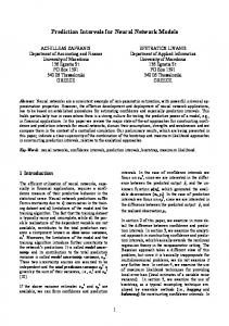
ANN for model development is the multilayer network shown in figure 1, known as the
SC
feedforward neural network. For model development using a multilayer feedforward neural network, the input variables are introduced to the network as a vector and are processed by the
M AN U
neurons of the first layer. Each neuron in the first layer is connected to all of the input variables and for each connection, a weight constant is assigned. The summation of all input variables multiplied by their respective weights and a bias constant yields the input of each neuron. A transfer function modifies the inputs to result the output of each neuron which is then transmitted
AC C
EP
TE D
to the neurons of the next layer to be processed further in the same way.
Figure 1- the configuration of a feedforward neural network
To develop an ANN model, the weights, biases and transfer functions are determined in a way that each set of inputs result in a final output equivalent to the required property. To do so, using a dataset with known input and output data (training dataset), the optimum values for the constants are determined through a procedure which is called the training of the network. Various training algorithms are developed and can be used for this purpose. With appropriate
2
ACCEPTED MANUSCRIPT
number of neurons, transfer functions and training algorithm, a multilayer feedforward ANN is capable of modeling any linear or non-linear correlation between the input and output variables12. Two widely used methods which apply ANNs to model chemical compounds properties in
RI PT
chemistry and chemical engineering are group contribution method (GCM) and quantitative structure property relationship (QSPR).
According to the GCM, properties of a compound are predicted based on the number and types
where
is the required property,
SC
of its constituting functional groups. The simplest form of a GCM based model has the form of:
and
(1)
are the number of presence and amount of
M AN U
contribution of functional group , respectively, and is a constant.
Prediction of properties via equation (1) is known as the Joback method. The Joback method typically produces poor results for large datasets. However, these results become considerably more accurate when the correlation between functional groups and the required property are mapped via ANNs. For example, using a feedforward neural network with one hidden layer containing 7 neurons, Albahri could predict the flash points of 375 transportation fuels based on
TE D
the GCM with an average absolute relative error (AARE) of 1.1 %, while the Joback method resulted an AARE of 4.3 % for the same dataset and functional groups 13. The group contribution based models which use ANNs have been widely used to predict various properties such as liquid viscosity
14-15
, thermal conductivity 16, infinite dilution activity 17, and
20
.
EP
density of ionic liquids 18, normal boiling point (NBP) 19, flash point (FP)
13
and melting point
AC C
Contrary to the classic GCM which only considers the functional groups as contributors to a property, the QSPR applies a more extensive set of structure based quantities, known as molecular descriptors, to model a property. To develop a QSPR model, the most effective molecular descriptors are screened from a pool of numerous calculated descriptors and are used as the inputs of the model. ANN based QSPR models have also been extensively used to predict various properties e.g. NBP 21, FP 22-24, surface tension 25, ideal gas entropy 26, aqueous solubility 27
, Hildebrand solubility parameter 28 and so on.
Using several available software tools e.g. Matlab, R, and Neurosolutions, developing an ANN model has become considerably straightforward, without requiring any knowledge of its 3
ACCEPTED MANUSCRIPT
extensive theoretical details. While simplified in practice, ANN models soon become unreliable without full consideration of important details e.g. appropriate assignment of the number of neurons, number of layers, and training of the network. More ever, selecting appropriate transfer function, training algorithm, dataset division and initialization of the network can also
RI PT
considerably improve the reliability and performance of an ANN model. The present study discusses such details and introduces the practical aspects of developing a robust ANN model. As a case study, predicting the flash point (FP) for an extensive dataset via a two layer feedforward neural network is investigated. The FP is one of the most important flammability , and its predictability via
M AN U
ANNs has been widely studied in many works 13, 30-32.
29
SC
properties of chemical compounds in assessment of fire hazards
2. Practical aspects of developing ANN models
2.1. Dataset division
The first step in developing an ANN model is to divide the dataset into three subsets, namely
TE D
training, validation and test datasets. The training dataset is used to train the network, where an error function which is usually the average absolute relative error or mean squared error is minimized with respect to the weight and bias constants in successive iterations. The number of compounds needed for training, as discussed later, is the first important factor affecting the
EP
reliability of an ANN model and determines the number of neurons and layers. As the training goes on, the performance of the ANN is continuously improved for the training
AC C
dataset, which simultaneously increases the risk of overfitting as well. Overfitting causes a model to yield accurate results for the dataset used for developing that model but poor results for the compounds out of this dataset. To prevent overfitting, the performance of the studied ANN is simultaneously monitored and validated for an independent dataset which is called the validation dataset. An increase in the error function of the validation dataset in several successive iterations is an indicator of overfitting and is used as a condition to stop the training. Once a neural network is trained, i.e. the optimum values of the weights and biases are determined, the performance of the ANN is examined using another independent dataset, known as the test dataset. Usually, 60-80 % of the dataset is assigned for training, 10-20% for validation and 104
ACCEPTED MANUSCRIPT
20% to test the model.
2.2. Assigning the number of neurons and hidden layers
RI PT
After specifying the training, validation and test datasets, selecting the number of layers, number of neurons in each layer, type of transfer functions and training algorithm and assigning the initial values for the weights and biases are the subsequent steps to develop an ANN model. The number of layers and neurons in each layer is one of the most crucial parameters affecting
SC
the performance and reliability of an ANN model. With a higher number of layers or neurons, an ANN typically yields more accurate results and can model more complicated relationships.
M AN U
However, this increase in the number of neurons or layers can also highly increase the risk of overfitting, simultaneously.
There are some recommendations to evaluate the appropriate number of hidden layer neurons, e.g. setting a number of hidden layer neurons equal to 2/3 of the number of input layer neurons 33
, between the number of neurons in the input and output layers
34
, or lower than twice the
number of neurons in the input layer 35. However, such recommendations don’t seem to be very
TE D
robust as they totally neglect the number of training samples and details of the ANN configuration as the most important factors.
Considering an ANN model as a regression problem, the ratio of the training samples to the total number of ANN constants as suggested by Jackson for regression models
36
, can be used as an
EP
index for determining the appropriate number of neurons and layers. For a multilayer feedforward neural network, if the number of input variables is , and the number of layers is
AC C
hidden layer is
, the number of neurons in the
, the total number of weight and bias constants
( ) can be calculated via:
=
+
!"
#
+
!
#
.
(2)
Obviously, the higher the ratio of the training samples to S, the higher the reliability of the results obtained by the model. It will be further discussed in section 4.2.
2.3. Assigning training algorithm and transfer function 5
ACCEPTED MANUSCRIPT
The applied transfer functions and training algorithm are also other ANN parameters which can have impacts on the performance of an ANN
37-38
. Some commonly used transfer functions in
ANN models which are also considered in our study are hyperbolic tangent sigmoid (tansig),
RI PT
log-sigmoid (logsig), Hard-limit (hardlim), Positive linear (poslin), and Radial basis (radbas) transfer functions for the hidden layers, and linear transfer function (purelin) for the output layer.
Table 1- Appropriate training algorithms in model development 39 Training algorithm
Abbreviation trainlm traingd trainrp trainscg trainbfg traincgf traingdm
TE D
2.4. Initialization of the network
M AN U
Levenberg-Marquardt backpropagation Gradient descent backpropagation Resilient backpropagation Scaled conjugate gradient backpropagation BFGS quasi-Newton backpropagation Conjugate gradient backpropagation with Fletcher-Reeves updates Gradient descent with momentum backpropagation
SC
The most widely used training algorithms are reported in table 1.
Assignment of the initial values for the weight and bias constants (initialization) is the last step before we can start training of the network. Initialization is a necessary task as the efficient training algorithms, all require some initial values for the weights and biases to optimize them in
EP
successive iterations via minimizing the error function. The error function which should be minimized with respect to the weight and bias constants, typically has several local minima. As a
AC C
result, starting from different initialization states determined by the initial values of the weights and biases, we may get to a quite different local minimum and obtain considerably different results. Some theoretical approaches on appropriate initialization of an ANN is reviewed by Yam and Chow
40
. An easy and yet very efficient approach to overcome the problems originated by
initialization is to repeat the training of the network for various initialization states 41, which will be taken in this work to show the effect and importance of initialization and also to overcome the discussed problems resulted by initializations.
2.5. Evaluating the reliable performance of an ANN model 6
ACCEPTED MANUSCRIPT
As discussed before and will be seen in the results, the performance of an ANN highly depends on the ANN specifications (applied dataset division, transfer function, training algorithm, initialization state and so on). Now the crucially important questions that arise are which ANN
Functional Group
provides the most reliable model and among all
RI PT
Table 2- The constituting functional groups used in group contribution method
different results which can be obtained via each ANN configuration using different initialization or dataset division states, which one represent the
–CH' – >CH– >C< ═CH' ═CH– ═C< ═C═ ≡CH ≡C– –OH –O– >C═O –CHO (aldehyde) –COOH (acid) –COO– (ester) HCOO– (formate) –NH' –NH– >N– ═N– –C≡N –NO' –F –Cl –Br –I –SH –S– –CH' – (ring) –HC< (ring) ═CH– (ring) >C< (ring) ═C< (ring) –O– (ring) –OH (ring) >C═O (ring) –NH– (ring) >N– (ring) ═N– (ring) –S– (ring) -CO-O-CO- (anidride)
authentic performance of that configuration? One
SC
2 3 4 5 6 7 8 9 10 11 12 13 14 15 16 17 18 19 20 21 22 23 24 25 26 27 28 29 30 31 32 33 34 35 36 37 38 39 40 41 42
may argue that the ANN which provides the most accurate results for the overall or test dataset is the
M AN U
–CH&
one to choose, however, such data won’t be reliable. An excellent performance for the overall dataset may be affected by overfitting and for the test dataset it can be just the result of a lucky dataset division. Another option is to use the average of results obtained for all studied
AC C
EP
TE D
1
initialization and dataset division states for an ANN. However, average of all results is not always informative because as discussed before, due to the high number of constants in many ANN models, error function typically has several local minima and therefore, initialization plays an important role. As a result, it is quite plausible that only a few initialization states may result in an accurate model (see e.g. the results obtained for developed FP predictive ANNs with 4 neurons, reported in the supplementary material) and therefore, the average of all results won’t represent the authentic performance of an ANN in most cases. In other words, a good initialization state may get lost 7
ACCEPTED MANUSCRIPT
among several other inappropriate initialization states by averaging. To overcome this issue, in the present study instead of averaging the results of all initialization and dataset division states, for each individual initialization state we retrain the model for several different dataset division states. The average of all obtained results are then considered as the
RI PT
authentic performance of that configuration. To find the most reliable model, the ANN for which in most of the repeats the observed errors of the training and test sets are not significantly different confirmed by available statistical tests, can be considered as the appropriately trained
SC
and reliable models..
M AN U
3. Material and method
3.1. Dataset
To develop a robust model, reliability of the dataset used for model development plays an important role. In the present study, the DIPPR 801
42
database was used to evaluate the
predictability of the FP for an extensive dataset of pure organic compounds. DIPPR 801 provides
predictive models.
TE D
evaluated data for several properties is one of the most widely used databases to develop FP
To implement a GCM based model, number of presence of the functional groups listed in table 2 and the experimentally determined data of the NBP were used as the inputs of the model. 43-46
EP
Normal boiling point and enthalpy of vaporization have been used is many FP predictive models , as both of them represent the volatility and hence, flammability of a fuel
47
. In previous
AC C
studies, it was shown that considering a contribution for the NBP in addition to the same functional groups listed in table 2, can significantly improve the predictability of the FP
43, 48
.
Among the organic compounds available in the DIPPR database, 740 compounds were available for which the reported data for both FP and NBP were experimentally determined. For other compounds, as a predicted data were reported for at least one of those properties, they were not considered in model development and evaluation. The full list of studied compounds can be found as supplementary material.
3.2. Initial implementation of the ANNs 8
ACCEPTED MANUSCRIPT
To study the various parameters affecting the performance of an ANN, the predictability of the FP for the dataset of 740 pure organic compounds from diverse families was initially investigated using feedforward neural networks with 1 to 10 neurons in the hidden layer. 75% of
RI PT
the dataset was assigned for training, 13% for validation, and 12% to test the ANN models.
To study the impacts of dataset division on the performance of ANNs, randomly division of the dataset was repeated 20 times. To investigate the impacts of various training algorithms, transfer functions and initialization states, for each dataset division the trainlm, traingd, trainrp, trainscg,
SC
trainbfg, traincgf, and traingdm training algorithms and tansig, logsig, hardlim, poslin, and radbas transfer functions were examined for 20 different initialization states. An increase in the
M AN U
mean squared error of the validation dataset in 6 successive iterations was considered as the condition to stop the training.
Therefore, considering 20 different dataset division states and for each one, assigning 1 to 10 neurons for the hidden layer, 5 different transfer functions, 7 different training algorithms, and 20 different initialization states, a total number of 140000 neural networks were initially implemented and their performance for FP prediction were evaluated using a Matlab code. The
TE D
performance of the ANNs were reported as percentage average absolute relative errors (AARE%) and correlation coefficients (R) defined as:
/ = ∑23)
AC C
EP
0
where )
*+,
and )
,-*.
-*4
78% = 0 ∑ :;
7=
−) >?@
B
"?@ ?@ @A>B >?@ @A>B ∑