3d part segmentation using simulated electrical charge ... - CiteSeerX

3D PART SEGMENTATION USING SIMULATED ELECTRICAL CHARGE DISTRIBUTIONS Kenong Wu and Martin D. Levine Centre for Intelligent Machines & Dept. of Electrical Engineering McGill University, Montreal, Quebec, Canada, H3A 2A7

Abstract A novel approach to 3D part segmentation is presented. Beginning with range data of a 3D object, we simulate the charge density distribution over an object's surface which has been tessellated by a triangular mesh. We then locate the object part boundary at deep surface concavities by tracing local charge density minima. Finally, we decompose the object into parts at the part boundary points.

1 Introduction

The problem of segmenting a 3D object into parts has attracted much attention in computer vision. The resolution of this problem is important for computing part-based descriptions and ecient object recognition [2, 12]. It has been customary to determine object parts by analysing geometrical properties of objects, such as surface curvature or volumetric shape. In this paper, we propose a novel approach to object segmentation into parts which is motivated by physics: An object to be segmented is viewed as a charged conductor. Thus a correspondence between the charge density distribution over the object's surface and the actual parts can be established. The object is then broken into parts based on the simulated charge density distribution on the object. Part segmentation algorithms can be categorised as being shape- or boundary-based. Shape-based approaches [12, 7, 9, 15] decompose objects into parts by measuring the shape similarity between image data and an arrangement of prede ned part models. In contrast, boundary-based methods segment objects into parts by seeking part boundaries instead of shape. Since this type of approach concentrates on part boundaries, it can segment an object without incorporating part shape information. For example, Koenderink and Van Doorn [10] have proposed parabolic lines as part boundaries. Rom and Medioni [13] have performed part decomposition based on this theory

using range data as input. Inspired by a particular regularity in nature - transversality, Homan and Richards [8] have proposed segmenting objects into parts at deep surface concavities. A few algorithms based on this concept have been developed to segment objects in range data [5, 4, 11]. The work reported in this paper is also boundarybased but employs a new surface property. Starting with single-view range data, we approximate an object surface by a triangular mesh and then simulate the electrical charge density distribution. We construct a Direct Connection Graph based on the triangular mesh, which provides a convenient coordinate system on the object's surface. Using this graph, we locate object part boundaries at deep surface concavities where the charge density achieves a signi cant local minimum. We then decompose the object into parts at the boundaries. There are certain advantages to our approach. Other boundary-based segmentation techniques are dominated by the need to analyse surface curvature. However, because of inherent input data noise and the necessity of computing derivatives, curvature computation has proven unreliable [16]. An assumption about surface smoothness is mandatory when using a curvature computation. In comparison, our approach involves the solution of a set of integral equations and therefore does not require such an assumption. Since the algorithm uses all data on the object's surface to compute the charge density at each location, the in uence of noise is greatly reduced.

2 Physics

When a charged conductor with an arbitrary shape is in electrostatic equilibrium, all charge resides unevenly on the outer surface of the conductor [3]. The charge density is very high at sharp convex edges and corners. Conversely, almost no charge accumulates at sharp concavities. Therefore deep surface concavities, which have been shown to delineate part bound-

O

O r

r

S

r Ti , fi =0

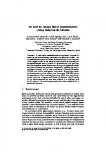
Figure 1: The observation point r and the charge source

point r on the surface S of an ellipsoid. O is the origin of the coordinate system.

Tk , fk =1

Figure 2: Triangular mesh on the surface of an ellipsoid.

0

aries [8], can be detected by isolating signi cant charge density minima. The physical model we have used is the charge density distribution on a perfect conductor in free space, where there is no other conductor or charge. Let r be a vector position of an observation point and r be a position of a source point charge q on the surface, as shown in Figure 1. Suppose charge is continuously distributed over the object surface S (see Figure 1). Then the electrical potential at r contributed by all of the charge on S can be expressed as follows [18]: 1 Z (r ) dS (r) = (1) 40 S jr ? r j Here (r ) is the charge density at r , S represents a unit area on S , and 0 is a constant, known as the permitivity of free space. According to physics [3], all points on a charged conductor in electric equilibrium are at the same electric potential. Since we restrict r in Equation (1) to the conductor surface, (r) is constant. Accordingly, (1) may be rewritten as follows: Z (r ) dS (2) V = 0

0

0

0

0

0

0

0

S

jr ? r j

0

0

Here V = 40 (r) is a constant. Since S in Equation (2) is an arbitrary surface, it is impossible to solve the equation analytically. However, we can obtain an approximate solution to Equation (2) by using nite element methods [14], as described in next section.

3 Finite Element Solution

To compute the charge density distribution based on Equation (2), the integration over the complete surface is converted to a summation of integrations over a number of planar triangles. These triangles form a triangular mesh tessellated on the object's surface. The mesh has N planar triangles, Tk ; k = 1; :::; N . Each

triangle is assumed to possess a constant charge density, k , as shown in Figure 2. A set of basis functions fk ; k = 1; :::; N is de ned on this triangular mesh as follows:  1 if r 2 Tk fk (r ) = (3) 0 otherwise The basis function, fk , is nonzero only when r (taken as the centroid of the triangular patch) is on the triangle Tk , as shown in Figure 2. Therefore, the charge density (r ) can be approximated by a piecewise constant charge density function as follows: N X k fk (r ) (4) (r )  0

0

0

0

0

0

k=1

Substituting (4) into Equation (2), we have N Z X 1 V = k jr ? r j dS 0

Tk

k=1

0

(5)

Since the charge density is assumed to be constant on each Tk , we may take ri as the observation point on each Ti and rewrite Equation (5) as: N Z X 1 V = k jr ? r j dS i = 1; ::::::; N: (6) k=1

Tk i

0

0

Because of charge conservation, the sum of the charges on each triangle equals the total charge on the surface of the conductor. Let Q be the total charge on the conductor and Sk be the area of Tk . Then we have N X Q= k Sk (7) k=1

Assuming Q is known, and using (6) and (7), we obtain a set of linear equations with N + 1 unknowns, 1 ; :::; N and V . Since the integral in (6) can be evaluated analytically [17], the charge density distribution k and the constant V can be obtained by solving a set of linear equations. This is accomplished using a conjugate gradient squared method [1].

3

6

6

6

1 4

7

2

4

7

2

5

8

(b)

3 4

7

(a)

1

8

(a)

5

(b)

5

(c)

Figure 3: Single-view range data of an object. (a) Frontal

Figure 5: Direct Connection Graph (DCG). (a) A triangular

4 Triangular Mesh Construction

5 Object Decomposition

view. (b) Side view. Due to self-occlusion, surface information on the other side cannot be seen by the laser range nder.

The charge density computation requires a closed triangular mesh to be tessellated on the complete surface of the object. However, the range data obtained from a particular view only re ect the visible surfaces, as shown in Figure 3. Thus it is impossible to perform the mesh tessellation based on the actual shape of the invisible parts of the object. In practice, we arti cially construct a mesh on the invisible side in order to make up a closed triangular mesh. This permits us to compute the charge density. We note that the actual shape of the invisible surface only aects the absolute value of the charge density on the visible surfaces. The position of the extrema of the charge density distribution remains almost the same and thus it makes sense to construct an arti cial mesh on the invisible surface. This argument is justi ed in [18]. The closed triangular mesh for the object is composed of three patches of triangular meshes, as shown in Figure 4. The rst, called the top patch, is obtained by triangulating the range data on the visible surface. The second, called the bottom patch, is planar, and is actually the (spatial) projection of the top patch onto an arbitrary plane perpendicular to the Z axis. These two patches are illustrated in Figure 4 (a). The third one , called the side patch, lls the gap between the top and the bottom patches, as shown in (b). The complete closed triangular mesh in Figure 4 (c) is obtained by merging the patches in (a) and (b). The details pertaining to the surface triangulation algorithm are given in [18].

(a)

(b)

(c)

Figure 4: Triangulation of the range data in Figure 3. (a) shows the top and the bottom patches of the closed triangular mesh. (b) shows the side patch. (c) gives the closed triangular mesh obtained by merging patches in (a) and (b).

mesh. (b) DCG of the triangular mesh in (a). (c) Subgraphs of (b) after boundary node deletion. Here triangular patches 1, 2, 3 and 8 are assumed to be located on the part boundary.

The object is decomposed into parts after obtaining the simulated charge density distribution. The method is based on a Direct Connection Graph(DCG) de ned on the triangular mesh, as shown in Figure 5. Here nodes represent triangular patches in the mesh and branches represent the connections between direct neighbours. Two triangles which share two vertices are considered to be direct neighbours. For example in Figure 5 (a), triangles 1 and 2 are direct neighbours while 2 and 3 are not. Thus the DCG provides a convenient coordinate system on the object surface and indicates the spatial relationship between a triangle and its neighbours. Object decomposition is performed by grouping triangles in the top patch of the closed mesh, which represents the visible surface. The strategy is to locate these triangles situated at part boundaries and then delete them from the graph. This divides the original DCG into a set of disconnected subgraphs, as shown in Figure 5 (c). Each object part represented by a subgraph can then be obtained by applying a component labelling algorithm to the DCG. The details regarding part boundary localisation can be found in [18].

6 Experimental Results

Before demonstrating part segmentation, we compare the noise sensitivities for the charge density and curvature computations. The latter has been traditionally used in boundary-based part segmentation [5, 4, 13]. In order to clearly illustrate the issues, we examine a simple 2D polygon, as shown in Figure 6. Due to the image sampling process, the boundary of this polygon is contaminated by high frequency noise. Figure 7 shows the computed charge density (the left column) and curvature (the right column). We use incremental curvature [6] to approximate the curvature of the jagged polygonal contour (increment = 1). In the rst row, although no smoothing has been applied to the polygon contour, the charge density clearly indicates both the concavities and convexities (see Fig-

Figure 6: A polygonal contour. Because of image quantisation, the boundary of the polygon in an image is jagged. 12

2.5

10

2

incremental curvature

charge density

6

4

(b)

(c)

(d)

Figure 8: A single view of a stone owl. (a) Shaded range data

of the owl. (b) The triangulartessellationon the visible surfaces. (c) The charge density distribution. (d) The segmented parts.

1.5

8

(a)

1

0.5

0

2

0 0

−0.5

50

100

150

300

350

400

−1 0

450

100

150

200 250 arc length

300

350

400

450

(b) 0.5

0.4

10

0.3

incremental curvature

12

8

6

0.1

0

2

−0.1

50

100

150

200 250 arc length

(c)

300

350

400

450

(a) (b) (c) (d) Figure 9: An alarm clock. (a) The shaded range data. (b)

0.2

4

0 0

50

(a)

14

charge density

200 250 arc length

−0.2 0

50

100

150

200 250 arc length

300

350

400

450

(d)

Figure 7: Comparison between charge density and curvature

computations. (a) and (b) show the computed charge density and curvature distributions, respectively, when no smoothing is applied to the contour shown in Figure 6. (c) and (d) illustrate the charge density and curvature distributions, respectively, when the contour is smoothed by a lowpass lter. These results indicate that the charge density computation is more robust than the curvature computation.

ure 7 (a)), while concave corners are very poorly indicated by the curvature distribution (see Figure 7 (b)). In the second row, we illustrate the experimental results produced by a smoothed polygonal contour. Here 2% of the energy of the highest Fourier frequency components of the jagged contour have been removed. It can be seen that the charge density distribution (see Figure 7 (c)) is much smoother than the curvature distribution (see Figure 7 (d)). These experiments clearly illustrate that the charge density computation is more robust with respect to high frequency noise than the curvature computation. The rst example of segmenting an object into parts involves the range data of a carved stone owl. Figure 8 (a) shows the shaded range data and (b) illustrates the triangular mesh for the visible surfaces. Here 368 triangular facets are used to represent the surface. The closed triangular mesh is composed of 966 triangles. Figure 8 (c) illustrates the computed charge density

The triangular tessellation for the visible surfaces. (c) The charge density distribution. (d) The segmented parts.

distribution on the surface. It can be clearly seen that the lowest charge densities are located at surface concavities. Conversely, the charge density at convexities exhibits a local maximum. As shown in Figure 8 (d), this object is segmented into three parts, namely, the head, the torso and the feet. In the second example, an alarm clock with two ringers on top is used. Figure 9 (a) and (b) show the shaded range data and the triangular mesh, respectively. There are 596 triangles tessellated on the visible surface and 1,878 triangles on the closed mesh. The computed charge density distribution is illustrated in Figure 9 (c) and the segmented parts are given in (d). Here the clock is decomposed into three parts. These results are consistent with our intuition of object parts. We note that although only partial shape information of the complete objects are available in these experiments, and the construction of the closed triangular meshes is rather arbitrary, our algorithm can still produce the desired results for the visible surfaces. Also, the relative sizes of the triangles is not crucial to the charge density computation. During our many experiments, we observed that even if the ratio of maximum to minimum triangle area was 200, our algorithm would still produce satisfactory results. The complexity of the charge density computation is governed by the construction of the coecient ma-

trix for the set of linear equations and the conjugate gradient squared method to solve the equation. The complexity of both is of the order of O(N 2), where N is the number of triangular facets. On a SGI R8000 workstation, the actual computing time for the charge distribution for the owl is 90 seconds, with about two seconds for surface triangulation, and one second for part decomposition.

7 Conclusions

This paper presents a new physics-based approach to 3D part segmentation. Unlike most previous approaches, which performed the surface curvature computation, we solve a set of integral equations over the whole object surface. Because of this, our algorithm does not require an assumption on surface smoothness and is robust to noise. Once segmented parts have been obtained, part-based descriptions can be computed [19] and utilised for ecient object recognition.

Acknowledgements We wish to thank Professor Jonathan Webb and Gilbert Soucy for their kind help. MDL would like to thank the Canadian Institute for Advanced Research and PRECARN for its support. This work was partially supported by a Natural Sciences and Engineering Research Council of Canada Strategic Grant and an FCAR Grant from the Province of Quebec.

References [1] R. Barrett, M. Berry, T. F. Chan, et al. Templates for the Solution of Linear Systems: Building Blocks for Iterative Methods. SIAM, Philadelphia, 1994. [2] I. Biederman. Human image understanding: Recent research and a theory. Computer Vision, Graphics, and Image Processing, 32:29{73, 1985. [3] F. J. Bueche. Introduction to Physics for Scientists and Engineers. McGraw-Hill Book Company, New York, 3rd edition, 1980. [4] F. P. Ferrie, J. Lagarde, and P. Whaite. Darboux frames, snakes and superquadrics: Geometry from the bottom up. IEEE Transactions on Pattern Analysis and Machine Intelligence, 15(8):771{784, August 1993. [5] F. P. Ferrie and M. D. Levine. Deriving coarse 3D models of objects. In Proceedings of IEEE Conference on Computer Vision and Pattern Recognition, pages 345{353, Ann Arbor, Michigan, June 1988. [6] H. Freeman. Shape descriptions via the use of critical points. Pattern Recognition, 10(3):159{166, 1978.

[7] A. Gupta and R. Bajcsy. Volumetric segmentation of range images of 3D objects using superquadric models. CVGIP: Image Understanding, 58(3):302{326, November 1993. [8] D. Homan and W. Richards. Parts of recognition. Cognition, 18:65{96, 1984. [9] T. Horikoshi and S. Suzuki. 3D parts decomposition from sparse range data using information criterion. In Proceedings of 1993 IEEE Computer Society Conerence on Computer Vision and Pattern Recognition, pages 168{173, New York City, NY, June 1993. IEEE Computer Society Press. [10] J. J. Koenderink and A. J. Van Doorn. The shape of smooth objects and the way contours end. Perception, 11:129{137, 1982. [11] A. Lejeune and F. Ferrie. Partioning range images using curvature and scale. In Proceedings of 1993 IEEE Computer Society Coonference on Computer Vision and Pattern Recognition, pages 800{801, New York City, NY, June 1993. IEEE Computer Society Press. [12] A. P. Pentland. Recognition by parts. In Proceedings of the First International Conference on Computer Vision, pages 8{11, London, June 1987. [13] H. Rom and G. Medioni. Part decomposition and description of 3D shapes. In Proceedings of the 12th International Conference on Pattern Recognition, volume I, pages 629{632, Jerusalem, Israel, October 1994. IEEE computer Society, IEEE Computer Society Press. [14] P. P. Silvester and R. L. Ferrari. Finite Elements for Electrical Engineering. Cambridge University Press, Cambridge, 2nd edition, 1990. [15] F. Solina, A. Leonardis, and A. Macerl. A direct partlevel segmentation of range images using volumetric models. In Proceedings of 1994 IEEE International Conference on Robotics and Automation, pages 2254{ 2259, San Diego, CA, May 1994. IEEE Robotics and Automation Society, IEEE Computer Society Press. [16] E. Trucco and R. B. Fisher. Experiments in curvaturebased segmentation of range data. IEEE Transactions on Pattern Analysis and Machine Intelligence, 17(2):177{181, February 1995. [17] D. Wilton, S. M. Rao, A. W. Glisson, et al. Potential integrals for uniform and linear source distributions on polygonal and polyhedral domains. IEEE Transactions on Antennas and Propagation, AP-32(3):276{ 281, 1984. [18] K. Wu. Computing Parametric Geon Descriptions of 3D Multi-Part Objects. PhD thesis, McGill University, Montreal, Canada, April 1996. [19] K. Wu and M. D. Levine. Recovering parametric geons from multiview range data. In Proceedings of IEEE Conference on Computer Vision & Pattern Recognition, pages 159{166, Seattle, June 1994.