Liver Segmentation Using Sparse 3D Prior Models with ... - CiteSeerX

Liver Segmentation Using Sparse 3D Prior Models with Optimal Data Support Charles Florin1 , Nikos Paragios2 , Gareth Funka-Lea1 , and James Williams3 1

Imaging & Visualization Department, Siemens Corporate Research, Princeton, NJ, USA 2

MAS - Ecole Centrale de Paris, Chatenay-Malabry, France 3

Siemens Medical Systems Forchheim, Germany

Abstract. Volume segmentation is a relatively slow process and, in certain circumstances, the enormous amount of prior knowledge available is underused. Model-based liver segmentation suffers from the large shape variability of this organ, and from structures of similar appearance that juxtapose the liver. The technique presented in this paper is devoted to combine a statistical analysis of the data with a reconstruction model from sparse information: only the most reliable information in the image is used, and the rest of the liver’s shape is inferred from the model and the sparse observation. The resulting process is more efficient than standard segmentation since most of the workload is concentrated on the critical points, but also more robust, since the interpolated volume is consistent with the prior knowledge statistics. The experimental results on liver datasets prove the sparse information model has the same potential as PCA, if not better, to represent the shape of the liver. Furthermore, the performance assessment from measurement statistics on the liver’s volume, distance between reconstructed surfaces and ground truth, and inter-observer variability demonstrates the liver is efficiently segmented using sparse information.

1 Introduction Computerized medical imaging analysis aims at detecting and delineating anatomical structures for surgery planning and diagnosis. It has gained significant importance in hepatic procedures, specially in oncology to detect tumors and lesions, quantify the ratio of tumors’ volume and liver’s volume (future liver remnant volume and total liver volume), their localization with respect to the liver’s vasculature and the different lobes of the liver [12][15]. Also, in the context of liver transplantation, graft from living donors is increasingly performed due to the shortage of cadaveric donors. This particular procedure requires a pre-operative quantification of the donor’s liver volume [6]. However, the segmentation of the liver is an arduous task for two main reasons. First, the liver’s appearance and shape has a large inter-patient variability; it is one of the largest organ of the human body, after the skin, and imaged patients may suffer from heavy diseases

such as cancer. Second, the neighboring structures have similar appearance in CT and MR, and may juxtapose the liver in a way that corresponds to a statistical shape variation, or without clear edge between the two. In this paper, we propose a novel method for liver segmentation that combines a statistical analysis of the data with a reconstruction model from sparse information: only the most reliable information in the image is used, and the rest of the liver’s shape is inferred from the model and the sparse observation. Given the difficulty of segmenting the liver, a model is commonly used, either as a localization, a shape or an appearance constrain. In [20], a cascading segmentation scheme sequentially detects the different abdominal structures for hepatic surgery planning. In [13][19], the liver is detected by a classification procedure based on the pixels intensity. A semiautomatic procedure is presented in [18] where a live-wire based on dynamic programming assists the user in drawing the liver’s contour slice by slice. In the context of deformable models, the reason for using prior knowledge is that this segmentation method is a local optimization, and therefore is sensitive to local minima. Therefore, the prior work on liver segmentation includes models based on shape variations, and constrains on pixel intensities learned from classification. Intensity based methods are used in [10] with snakes segmenting the liver’s contour in a slice-by-slice fashion. However, the vicinity of the liver to neighboring structures of similar appearance makes models attractive for this task [5]. The models used in [5] are based on Cootes et al.’s Active Shape Models [1]. The results obtained in [5] demonstrate Active Shape Models may represent to a certain extent the liver’s shape. However, they fall short of accurately segmenting the liver because of the large shape variability of this organ. Furthermore, Active Shape Models are highly dependent on initialization, a problem the authors deal with using multi-resolution. Nonlinear models, such as shapebased Kernel PCA [2] or Fourier coefficients [3], are also a solution that have been investigated more recently for segmentation. The main limitation of these methods (linear or non-linear) is the explicit assumption of the data distribution that, for example, forms a linear subspace in the case of PCA. These methods process the total amount of data and find the optimum trade-off between an image term and a prior term. Furthermore, the quality of image support is at no point taken into account; it is assumed that should an image region quality be low, another region would compensate. Most of these methods treat segmentation as a statistical estimation problem, where the quality and the support of the training set’s exemplars is often ignored. Instead, the approach presented in this paper relies on observation at key locations, and on a reconstruction model ; both the key locations and the reconstruction models are learned from prior knowledge. This technique gives better results because the segmentation is only supported by the data with the strongest image support, and is also of low complexity because it uses the data in an optimal fashion. Interpolation models have been studied before. The simplest and most common method is to use a spline or piecewise polynomial function [14, 21] that interpolates the contour between explicit points. Other methods use an implicit representation of the contour (a continuous function that takes a zero value on the contour) and interpolating functions such as thin-plate splines [22]. An example of surface reconstruction is the work of Hoppe et al. [7] who computed a signed distance function in 3D which is

the distance in R3 to any input point. Then, from the zero levelset of this function is extracted the surface using the Marching Cubes [11]. At last, deformable models [9] are used to minimize an energy function of the mesh by deforming the mesh so that the mesh is simultaneously attracted to the data by an image term, kept smooth by a tension term and by an optional prior term. The approach we propose here is different: we propose a liver model that encodes the shape variations using a small number of carefully chosen key-slices where the organ’s contours can be optimally recovered. First, the image or shape to reconstruct is discretized along the longitudinal axis, and all the liver exemplars are registered so that they fit into the same reference region. Then, a set of slice indices are determined so that it minimizes three different criteria: image support, quality of the reconstruction and sensibility to variations in the projection’s subspace. Finally, the reconstruction operator itself is learned over the given liver exemplars. To present this approach, section (2) contains a rather generic formulation of Sparse Information Models. Then, section (3) is devoted to explicit this model to the particular problem of 3D liver segmentation. To validate the methodology, section (4) aims at proving the liver’s shape is indeed well recovered from few contours at key-slices, and quantifying the quality of the segmentation obtained in this way.

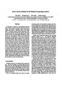
2 Choice of Sparse Information Let us consider a shape x and its partition into m elements x = (x1 , ..., xm ) (see figure (1)) associated to m measures w = (w1 , ..., wm ) which reflect the data support for the observations. Without loss of generality, we assume the m sub-elements are obtained by a discretization process along one or several axis v0 using an operator ρ : [Ωr × R] → Ωr /v0 : ∀ k ∈ [1, m], xk = ρ(x, k) (1) In the remaining of the paper, this continuous parameterization is assumed when not specified. The aim of our approach is to recover a minimal description length set of |B| sub-elements B = {xtk }k∈[|1,K|] with K small compared to m, and a continuous operator φ, from which the whole data x is deducted: ∀ k ∈ [1, m], φ(xt1 , ..., xtK , k) = x(k).

(2)

2.1 Optimal Reconstruction of the Data Let us consider a training set of P exemplars X = {x1 , x2 , ..., xP } registered in a reference space Ωr . Toward optimal reconstruction of the training set from the basis B, the distance between the reconstruction and the existing samples is minimized. To this end, let a metric ψ : [Ωr × Ωr ] → R+ measures the distance between two subelements. Then, assuming the number of components of the training set is fixed, such reconstruction minimizes Eint (B, φ) =

P X m X p=1 i=1

¡ ¢ ψ xpi , φi (xpt1 , ..., xptK ) .

(3)

Fig. 1. Example of a 3D liver surface x whose subcomponents (x1 , ..., xm ) are obtained by intersecting the 3D shape with the axial plane (dark contours) at specific slice indices s1 , s2 , ...sK .

Such an approach is purely geometric and does not account for the image support of each sub-element. 2.2 Optimal Image Support We recall that the sub-elements of a given exemplar xp have some underlying image p support noted wp = (w1p , ..., wm ). The optimum basis B consists of elements that are confidently extracted from the data; therefore, the basis minimizes Esup (B) =

P X K X ¡ ¡ ¢¢ g wkp Tθ−1 (xptk )

(4)

p=1 k=1

where g is a monotonically decreasing function, and Tθ−1 (xptk ) is the inverse mapping between the basis B and the observation space. The use of such inverse mapping is also to be considered during the application of the model to new data. Therefore, it is critical to have a selection of B that is relative robust to errors when locating the basis elements in a new exemplar. 2.3 Robustness to Parameters Variability Let us consider a slight variation on the selection of the basis, noted δxt . For the interpolation precision of the model not to be significantly affected, lim Eint (B, φ) − Eint (B + δxt , φ) =0 |δxt | → 0 δxt

(5)

that is reformulated in terms of a cost by defining a smoothness function η(), like the error-two norm, Evar (B, φ) = η (∇B Eint (B, φ)) . (6)

Such a penalty term introduces robustness in the basis selection step, as well to the reconstruction process. Now, one integrates these three constraints into a single cost function: E(B, φ) = Eint (B, φ) + αEsup (B) + βEvar (B, φ) where α and β are problemspecific normalizing constants (results have shown little sensibility to small variations of α and β). The cost function E is minimized with respect to the interpolation function φ and the basis B. Such a process cannot be described in a general fashion, but a gradient descent is an excellent choice when considering linear interpolation models, while more advanced non-linear optimization methods like neural networks can be considered for non-linear cases. Last, but not least the residual cost that characterizes the Sparse Information Model is used to determine the best number K of key components that optimizes the Minimum Description Length. In order to demonstrate the efficiency of such a model for volumetric organ segmentation, we consider the particular case of liver segmentation in CT images. The same approach is easily adapted to any other organ, in any dimension.

3 Sparse Knowledge-based Segmentation Knowledge-based segmentation is one of the dominant approaches to organ extraction from 3D images. First, the Sparse Model is built by selecting a minimal set B of 2D contours (represented in an explicit or an implicit fashion) along with an interpolation function φ to reconstruct the whole 3D surface in the reference space Ωr . During the segmentation, the global transformation Tθ that relates the reconstructed model to the observation volume is to be determined, along with the set B of 2D contours that fits the observation. 3.1 Model Construction The experiment is conducted on segmentation for medical imaging for the case of liver in Computed Tomography (CT). We represent the training set exemplars x by 3D distance maps to the closed surface Γ defined by the liver’s edge C in the volumetric data:  0, p ∈ C   ∀p ∈ Ω, x(p) = +D(p) ≥ 0, p ∈ Γ (7)   ¯ −D(p) < 0, p ∈ Γ Such a selection is motivated from its implicit nature, as well as the ability to introduce surface-based as well as area based criteria in the segmentation process. Classic explicit parameterizations like triangulated surfaces, or other form of parametric snakes can also be considered. The acquisition process guides our choice for the definition of the sub-elements: since the image volume is reconstructed slice by slice, with maximum resolution in the slice plane, the axis of projection vi0 (see section (2)) is the longitudinal axis. Therefore, a sub-element xi corresponds to a particular slice (see figure (1)). The geometric transformation Tθ is a translation-scaling that sets x in a reference space Ωr with m slices (x1 , ...xm ).

In order to determine the best possible interpolation class, different models for φ have been tested. We have concluded that generalized linear interpolation for each slice i is a good compromise between complexity and interpolation quality. In other words, the solution (2D contour) at each slice xi is reconstructed using a particular linear combination Hi of the key contours xt1 , ...xtK . This notation is kept in the remaining of the paper: φ = H. The interpolation quality is defined according to sum of square difference between the reconstructed distance map and the observed shape’s distance map in the reference space Ωr : m Z ¯ ¯2 X ¯ ¯ T Eint (B, H) = (8) ¯Hi [xt1 , ...xtK ] − xi ¯ i=1

Ωr

Eint is a quadratic function with global minimum, and since the reference space Ωr is a continuous space, the minimization of Eint benefits from the large literature on quadratic functions minimization. The image support wi at slice i is defined by the Kullback-Leibler distance between the pixels intensity distributions inside and outside the 2D contour and the a priori learned histograms. Knowing a priori the normalized histogram hin (resp. hout ) of the pixels intensity inside (resp. outside) the liver, and computing the pixels intensity distribution pin and pout inside and outside of the reconstructed shape on the key slices, µ ¶ µ ¶ K Z K Z X X hin (k, s) hout (k, s) Esup (B) = hin (k, s)log ds+ hout (k, s)log ds. pin (k, s) pout (k, s) k=1 k=1 (9) Finally, the key contours are chosen so as to minimize the impact of little variations in their position, and of little errors in the contours extraction in the key slices. Since a continuous interpolation of the 2D contours is introduced in equation (1), the impact of an infinitesimal change ∂k in the slice index may be written as the squared magnitude 2 of the gradient of xtk with respect to tk : k∇tk xtk k . In practice, since the contours are represented using distance functions (see equation (7)), the derivative of the distance function at index tk , with respect to the index, is a field of 2d vectors whose squared 2 magnitude is k∇tk xtk k . Therefore, the key contours are chosen so as to minimize the integral over the image space of the distance map’s gradient at the key locations: K Z X 2 Evar (B) = k∇tk xtk k . (10) k=1

Ωr

In order to determine the number K, the indices of the key contours t1 , ...tK as well as the interpolation operator H, a gradient descent optimization method is used and combined with the Schwarz Bayesian criterion [4] to determine the optimum cardinality of the basis. After registering the volumes with m = 100 slices, the optimum number of key slices is 5. 3.2 Model-based Segmentation With sparse model in hand, the volumetric segmentation is boiled down to the segmentation of the shape at key slices; in other words, the whole 3D segmentation problem

is reduced to a small set of parallel 2D contours to be segmented at specific locations. Therefore, one needs to optimize an image-based cost function with respect to both the set of key contours B = xt1 , ...xtK in the reference space and the transformation Tθ simultaneously. In an iterative optimization scheme, the transformation Tθ at a given iteration is used to relate the current set of 2D contours xt1 , ...xtK to the image so that both the transformation and the sparse set of contours are optimized concomitantly. To this end, the cost function consists of the intensity-based likelihood of each pixel, assuming that normalized histograms inside (hin ) and outside (hout ) the liver are available (if not, one recovers them on-the-fly). Then, the posterior likelihood of the partition with respect to the two classes is maximized to obtain the key contours B and the transformation Tθ : K Z X ¡ ¢ Eseg (B, Tθ ) = −log hin (I(s)) H(xtk (Tθ (s))) ds +

K Z X k=1

Ω

k=1

Ω

(11)

−log (hout (I(s))) (1 − H(xtk (Tθ (s)))) ds,

where H(xtk (s)) denotes the Heaviside function that is equal to 1 inside the contour xtk , and 0 outside. During the sparse model’s construction the image support has been taken into account in the selection of the key slices. This information has been inherited to the segmentation and, in principle, the slices where one best separates liver from the rest of the background are used (see equation (9)). When (B, Tθ ) have reached the energy minimum, the whole volumetric shape x is reconstructed in Ωr by applying the linear combination Hi for each slice i. Finally, the inverse of Tθ is used to transform the reconstructed volume from Ωr to the image space Ω. In a subsequent step, one may consider refining the results by locally optimizing the solution x on each slice i, using the sparse model’s result as a prior such as [17].

4 Experimental Validation 4.1 Dimensionality Reduction using Sparse Information Model Before proving Sparse Information Models are efficiently used to segment an organ in volumetric data, one needs to quantify the error introduced by the Sparse Models dimension reduction and compare it with common techniques such as PCA. The volumetric data is acquired on Sensation 16 CT scanners, with an average resolution of 1 mm in axial plane and 3 mm along the longitudinal axis. 31 volumes (different oncology patients, with or without pathologies such as tumors) are used in our experiments on a leave-one-out basis: 30 volumes are used to build the models (sparse and PCA) and the last one is used for testing. Table (1) summarizes the error introduced by dimensionality reduction for PCA (30 modes), linear interpolation and Sparse Information Model with 5 slices. This error measure is defined as the symmetric difference [18] between the two volumes V1 and V2 : |V1 ∩ V2 | (12) ²=1− 0.5 ∗ (|V1 | + |V2 |)

method median symmetric diff. maximum symmetric diff. minimum symmetric diff.

PCA Linear interp. 11.70% 10.72% 23.32% 16.13% 6.56% 7.69%

SIM 8.35% 13.14% 6.28%

Table 1. Results table showing the median, maximum and minimum symmetric difference between ground truth volumes and reconstructed volumes using PCA (30 modes), linear interpolation from 5 key slices and Sparse Information Model (SIM) with 5 key slices.

The results demonstrate that the Sparse Information Model with 5 key elements provides the same reconstruction quality than linear PCA with 30 modes of variation. However, the PCA results have a large variance because diseased organs are poorly represented by a Gaussian model in the linear PCA space. Nevertheless, a larger study with different pathologies could demonstrate kernel PCA [8] best represents the shapes. Figure (2) illustrates different error measures for liver segmentation with linear PCA, liner interpolation and Sparse Information Model. The quality assessment is performed with four error measures: the volumetric error in %, the average surface distance, the RMS distance, and the percentage of surface father than 5mm from the ground truth. 4.2 Sparse Information Model for Segmentation The second step consists in demonstrating Sparse Information Models can efficiently be used for segmentation. For that purpose, it is assumed an expert (i.e. either a human expert, or an expert system such as the ones described in the literature) roughly initializes the rigid transformation and the key contours. When no user interaction is available, a preprocessing step, such as exhaustive search or coarse-to-fine search, is to be developed. In the case of PCA [16], the segmentation problem is solved by minimizing the cost function resulting from the intensity-based likelihood of each pixel in the volumetric image: Eseg = +

m Z X k=1

Ω

m Z X k=1

Ω

¡ ¢ −log hin (I(s)) H(xk (Tθ (s))) dΩ (13)

−log (hout (I(s))) (1 − H(xk (Tθ (s)))) dΩ,

As in [16], equation (13) is minimized in the PCA’s parametric space, where the shapes’ distribution is modeled using kernels. The kernels are justified by the poor modeling of the samples distribution by a Gaussian. For the PCA segmentation, all the m slices of the volume are used, whereas the Sparse Information Model only segments the K slices determined during the model construction (see equation (11)). Table (2) summarizes the symmetric difference (see equation (12)) between ground truth and the segmented liver obtained using the Sparse Information Model and PCA [16] (see figure (3)). Neighboring structures of similar intensities juxtapose the liver in a way that PCA estimates as a shape variation. On the contrary, the Sparse Model ignores the regions with low support, and reconstructs the information in these regions based on

Volumetric error [%]

Avg. Distance [mm]

RMS Distance [mm]

Deviations > 5mm [%]

Fig. 2. Segmentation result boxplots comparing PCA (5 and 30 modes), linear interpolation and Sparse Information Model. The box has lines at the lower quartile, median, and upper quartile values. The whiskers are lines extending from each end of the box to show the extent of the rest of the data. Outliers are data with values beyond the ends of the whiskers.

other visual clues elsewhere in the image. For information, the inter-observer symmetric difference in table (2) indicates the symmetric difference between livers segmented by different experts using the same semi-automatic tool. Overall, when compared with [5], the results seem to demonstrate Sparse Information Models outperform Active Shape Models. Nevertheless, it must be underlined that the training and evaluation datasets are different. Furthermore, in [5], the shape model is built from smoothed surface meshes, while the training shapes used in this paper are represented by distance functions (see equation (7)) and are not smoothed. However, as one suspects, Sparse Information Models are sensitive to initialization. To quantify this, two different Sparse Segmentations were performed by segmenting by hand the key slices in the datasets, and comparing the reconstruction results with the ground truth. The difference in quality (symmetric difference with ground truth) between the different reconstructions ranges from 0.02% to 6.73%. Moreover, this variance is not correlated to the IOV (correlation coefficient of 0.47); otherwise stated, a volume with high inter-observer variability may be segmented by the SIM in a way that is robust to initialization, and reciprocal may be true. Indeed, the IOV depends on the whole organ’s structure while the SIM’s quality only depends

method median symmetric diff. maximum symmetric diff. minimum symmetric diff.

PCA 26.41% 36.84% 16.68%

SIM 11.49% 17.13% 9.49%

IOV 5.56% 7.83% 2.96%

Table 2. Results table showing the average symmetric difference and maximum symmetric between hand-segmented livers and automatic segmentation with PCA and Sparse Information Model (SIM). Also, is also given the Inter-Observer Variability (IOV) statistics.

on the key slices. Furthermore, the maximum quality difference of 6.73% is below the maximum IOV symmetric difference (7.83% in table (2)).

5 Conclusion In this paper, we have introduced a novel family of dimension reduction techniques based on intelligent selection of key sub-elements with respect to reconstruction quality, image support and variability of these key sub-elements. It is demonstrated that Sparse Information Models can be used for dimensionality purposes, and can efficiently be integrated into a segmentation framework in the context of volumetric organ segmentation. We have applied this technique to the problem of liver segmentation in volumetric images with successful results compared to common dimensionality reduction techniques based on linear projections and kernel distributions. On top of interpolation and segmentation quality, this method is also very fast since only the most important and most reliable information is processed for the reconstruction of the whole information. However, as noted in [5], a statistical shape model may not be sufficient to represent the exact shape of the liver ; in a post-processing step, a local optimization - using active contours for instance - may be necessary for better results. This local optimization would not be computed from Sparse Information. Further work will investigate the use of non-linear models for the interpolation function, as well as a subsequent refinement step that will locally adjust the reconstruction from the model to the actual image information by taking into account the confidence in the reconstruction. More advanced prior models using axial coronal and sagittal sparse information would be an interesting extension of our approach, as it would diminish the quality difference between two differently initialized segmentations. Last, but not least, the use of such methods for feature extraction, classification and content-based image indexing and retrieval is a natural extension on the application side.

References 1. T. Cootes, C. Taylor, D. Cooper, and J. Graham. Active shape models - their training and application. Computer Vision and Image Understanding, 61:38–59, 1995. 2. S. Dambreville, Y. Rathi, and A. Tannenbaum. Shape-based approach to robust image segmentation using kernel pca. In CVPR, pages 977–984, Washington, DC, USA, 2006. 3. S. Derrode, M. Chermi, and F. Ghorbel. Fourier-based invariant shape prior for snakes. In ICASSP, 2006. 4. M. H. Hansen and B. Yu. Model selection and the principle of minimum description length. Journal of the American Statistical Association, 96(454):746–774, 2001.

5. T. Heimann, I. Wolf, and HP. Meinzer. Active shape models for a fully automated 3d segmentation of the liver - an evaluation on clinical data. In MICCAI (2), pages 41–48, 2006. 6. L. Hermoye, I. Laamari-Azjal, Z. Cao, L. Annet, J. Lerut, B. Dawant, and B. Van Beers. Liver segmentation in living liver transplant donors: comparison of semiautomatic and manual methods. Radiology, 234(1):171–178, January 2005. 7. H. Hoppe, T. DeRose, T. Duchamp, J. McDonald, and W. Stuetzle. Surface reconstruction from unorganized points. In SIGGRAPH ’92: Proceedings of the 19th annual conference on Computer graphics and interactive techniques, pages 71–78, 1992. 8. M. Leventon, E. Grimson, and O. Faugeras. Statistical Shape Influence in Geodesic Active Controus. In IEEE Conference on Computer Vision and Pattern Recognition, pages I:316– 322, 2000. 9. CW. Liao and G. Medioni. Surface approximation of a cloud of 3d points. Graph. Models Image Process., 57(1):67–74, 1995. 10. F. Liu, B. Zhao, P. Kijewski, L. Wang, and L. Schwartz. Liver segmentation for ct images using gvf snake. Medical Physics, 32(12):3699–3706, December 2005. 11. W. Lorensen and H. Cline. Marching cubes: A high resolution 3d surface construction algorithm. In SIGGRAPH ’87: Proceedings of the 14th annual conference on Computer graphics and interactive techniques, pages 163–169, New York, NY, USA, 1987. ACM Press. 12. HP. Meinzer, M. Thorn, and C. Cardenas. Computerized planning of liver surgery-an overview. Computer and Graphics, 26(4):569–576, August 2002. 13. H. Park, P. Bland, and C. Meyer. Construction of an abdominal probabilistic atlas and its application in segmentation. IEEE Trans. Med. Imaging, 22(4):483–492, April 2003. 14. B. Pham. Quadratic b-splines for automatic curve and surface fitting. C&G, 13:471–475, 1989. 15. B. Reitinger, A. Bornik, R. Beichel, and D. Schmalstieg. Liver surgery planning using virtual reality. IEEE Comput. Graph. Appl., 26(6):36–47, 2006. 16. M. Rousson and D. Cremers. Efficient kernel density estimation of shape and intensity priors for level set segmentation. In MICCAI (2), pages 757–764, 2005. 17. M. Rousson and N. Paragios. Shape Priors for Level Set Representations. In European Conference on Computer Vision, pages II:78–93, Copenhangen, Denmark, 2002. 18. A. Schenk, G. Prause, and HO. Peitgen. Efficient semiautomatic segmentation of 3d objects in medical images. In MICCAI, pages 186–195, 2000. 19. KS. Seo, HB. Kim, T. Park, PK. Kim, and JA. Park. Automatic liver segmentation of contrast enhanced ct images based on histogram processing. In ICNC (1), pages 1027–1030, 2005. 20. L. Soler, H. Delingette, G. Malandain, J. Montagnat, N. Ayache, C. Koehl, O. Dourthe, B. Malassagne, M. Smith, D. Mutter, and J. Marescaux. Fully automatic anatomical, pathological, and functional segmentation from CT scans for hepatic surgery. Computer Aided Surgery (CAS), 6(3), August 2001. 21. S. Tehrani, T.E. Weymouth, and B. Schunck. Interpolating cubic spline contours by minimizing second derivative discontinuity. ICCV, pages 713–716, 90. 22. G. Turk and J. O’brien. Modelling with implicit surfaces that interpolate. ACM Trans. Graph., 21(4):855–873, 2002.

Fig. 3. Comparison of liver segmentation obtained by SIM (left column) and expert segmentation (right column).