3D Person Tracking with a Color-Based Particle Filter - Informatik 12

3D Person Tracking with a Color-Based Particle Filter Stefan Wildermann and J¨urgen Teich Hardware/Software Co-Design, Department of Computer Science, University of Erlangen-Nuremberg, Germany {stefan.wildermann, juergen.teich}@informatik.uni-erlangen.de

Abstract. Person tracking is a key requirement for modern service robots. But methods for robot vision have to fulfill several constraints: they have to be robust to errors evoked by noisy sensor data, they have to be able to work under realworld conditions, and they have to be fast and computationally inexpensive. In this paper we present an approach for tracking the position of a person in 3D based on a particle filter. In our framework, each particle represents a hypothesis for the 3D position, velocity and size of the person’s head being tracked. Two cameras are used for the evaluation of the particles. The particles are weighted by projecting them onto the camera image and applying a color-based perception model. This model uses skin color cues for face tracking and color histograms for body tracking. In contrast to feature-based approaches, our system even works when the person is temporary or partially occluded.

1

Introduction

New scenarios for service robots require sophisticated ways for users to control robots. Since such systems are designed to support humans in everyday life, special user interfaces, known as Human Machine Interfaces (HMIs), have to be developed that support the cooperation, interaction and communication between robot and user. A basic requirement for a proper HMI is the awareness of the person that is currently interacting with it. Methods for robot vision have to fulfill several constraints. First, they have to be robust to errors evoked by noisy sensor data, changing lighting conditions, etc. Second, they have to be able to work under real-world conditions with moving objects and persons. Moreover, adequate algorithms have to be computationally inexpensive and fast, since a robot has to simultaneously perform several tasks. Tracking algorithms can be divided into two classes. In bottom-up approaches the camera images are searched for significant features of persons such as the face. The detected features are then used for tracking. In contrast, top-down approaches make assumptions of the possible position of the person. These hypotheses are then evaluated by considering the current camera images. Usually, such approaches are faster than algorithms of the first class, since the images have only to be processed on the hypothetical positions. Service robots have to deal with highly dynamic environments. This implies the use of adaptive methods. In recent years, probabilistic approaches have proven to be appropriate for such tasks, and thus have become quite popular in robotics [1]. The key

G. Sommer and R. Klette (Eds.): RobVis 2008, LNCS 4931, pp. 327 – 340, 2008. c Springer-Verlag Berlin Heidelberg 2008

idea of the presented system is to use a particle filter as the probabilistic framework for a top-down approach. Particles represent hypotheses for the person’s position in 3D coordinates. In order to evaluate these particles, they are projected onto the image planes. The probability for observing the person at the resulting image coordinates is then calculated according to a color-based perception model. This model uses skin color cues for face tracking and color histograms for body tracking. Furthermore, a method for an automatic initialization of the tracker is provided. The further outline of this paper is as follows. In Section 2 we will give an overview of related work. Then, in Section 3 probabilistic tracking is briefly described. Section 4 outlines the system proposed in this paper. The color-based perception model is presented in Section 5. Section 6 shows, how the tracker can be properly initialized. In Section 7 the results are presented that were achieved with the tracker. We conclude our paper with Section 8.

2

Related Work

Person tracking plays an important role for a variety of applications, including robot vision, HMI, augmented reality, virtual environments, and surveillance. Several approaches based on a single camera exist for this task. Bottom-up approaches for person tracking are based on feature extraction algorithms. The key idea is to find significant features of the human shape that can be easily tracked such as, e.g, eyes or the nose [2], but most algorithms rely on face detection. Color can provide an efficient visual cue for tracking algorithms. One of the problems faced here is that the color depends upon the lighting conditions of the environment. Therefore statistical approaches are often adopted for color-based tracking. Gaussian mixture models are used to model colors as probability distributions in [3] and [4]. Another approach is to use color histograms to represent and track image regions. In [5] color histogram matching is combined with particle filtering, thus improving speed and robustness. In recent years, a number of techniques have been developed that make use of two or more cameras to track persons in 3D. Usually, stereo vision works in a bottom-up approach. First, the tracked object has to be detected in the images that are simultaneously taken by at least two calibrated cameras. The object’s 3D position is then calculated via stereo triangulation [6, 7]. The main problems of bottom-up approaches are that the object has to be detected in all camera images and the detected features have to belong to the same object known as the correspondence problem. If this is not the case, the obtained 3D position is erroneous. In [8, 9] particle filters are applied to track persons in 3D using a top-down approach. Each particle is evaluated for all available cameras by using cascaded classifiers as proposed by Viola and Jones [10]. The disadvantage of these approaches is that they fail to track an object when it is partially occluded which is often the case in real world applications. The approach described in this paper overcomes this drawback by using a color-based algorithm. We will show that our method is able to track people even when they are temporarily and partially occluded. DOI: 10.1007/978-3-540-78157-8 http://www.springerlink.com/content/x80x381762364902/

G. Sommer and R. Klette (Eds.): RobVis 2008, LNCS 4931, pp. 327 – 340, 2008. c Springer-Verlag Berlin Heidelberg 2008

3

Bayesian Tracking

The key idea of probabilistic perception is to represent the internal view of the environment through probability distributions. This has many advantages, since the robot’s vision can recover from errors as well as handle ambiguities and noisy sensor data. But the main advantage is that no single ”best guess” is used. Rather, the robot is aware of the uncertainty of it’s perception. Probabilistic filters are based on the Bayes filter algorithm whose basics with respect to probabilistic tracking will be briefly described here. For a probabilistic vision-based tracker the state of an object at time t is described by the vector xt . All measurements of the tracked object since the initial time step are denoted by z1:t . The robot’s belief of the object’s state at time step t is represented by the probability distribution p(xt |z1:t ). This probability distribution can be rewritten using the Bayes rule p(xt |z1:t ) = We now define η =

p(xt |z1:t )

1 p(zt |z1:t−1 )

p(zt |xt , z1:t−1 )p(xt |z1:t−1 ) . p(zt |z1:t−1 )

(1)

and simplify Equation 1:

η p(zt |xt , z1:t−1 )p(xt |z1:t−1 )

(2)

Markov

=

η p(zt |xt )p(xt |z1:t−1 )

(3)

Total Prob.

Z

=

=

Markov

=

η p(zt |xt ) η p(zt |xt )

Z

p(xt |xt−1 , z1:t−1 )p(xt−1 |z1:t−1 )dxt−1

(4)

p(xt |xt−1 )p(xt−1 |z1:t−1 )dxt−1

(5)

In Equation 3 the Markov assumption is applied which states that no past measurements z1:t−1 is needed to predict zt if the current state xt is known. In Equation 4 the probability density p(xt |z1:t−1 ) is rewritten by using the Theorem of total probability. Finally, in Equation 5 the Markov assumption is exploited again since the past measurements contain no information for predicting state xt if the previous state xt−1 is known. The computation of the integral operation in Equation 5 is very expensive, so several methods were developed to estimate the posterior probability distribution efficiently, such as the Kalman filter or the Information filter. These filters represent the posterior as a Gaussian which can be described by the first two moments i.e., its mean and covariance. But most real-world problems are non-Gaussian. So non-parametric probabilistic filters, such as Particle filters, are better suited to such tasks [11]. Different from parametric filters, the posterior probability distribution p(xt |z1:t ) is not described in a functional form, but approximated by a finite number of weighted samples with each sample representing a hypothesis of the object’s state, and its weight reflecting the importance of this hypothesis. These samples are called particles and will be denoted as xti with associated weights wti . DOI: 10.1007/978-3-540-78157-8 http://www.springerlink.com/content/x80x381762364902/

G. Sommer and R. Klette (Eds.): RobVis 2008, LNCS 4931, pp. 327 – 340, 2008. c Springer-Verlag Berlin Heidelberg 2008

The particle filter algorithm is iterative. In each iteration, first n particles are sampled from the particle set Xt = {hxti , wti i}i=1...n according to their weights and then propagated by a motion model that represents the state propagation p(xt |xt−1 ). The resulting particles are then weighted according to a perception model p(zt |xt ). A problem of particle filters is the degeneracy problem standing for that after a few iterations all but one particle will have a negligible weight. To overcome this problem generic particle filter algorithms measure the degeneracy of the algorithm with the effective sample size Ne f f introduced in [12] and shown in Equation (6). N

Ne f f = 1/ ∑ (wti )2 .

(6)

i=1

If the effective sample size is too small, there will be a resampling step at the end of the algorithm. The basic idea of resampling is to eliminate particles with small weights and to concentrate on particles with large weights. The purpose of this paper is to show, how to use this probabilistic framework to track a person in 3D.

4

Top-Down Approach to 3D Tracking

The aim of the system presented here is to track the coordinates of a person in 3D. The position of the person’s head p = (x, y, z)T serves as reference point for our person model. Furthermore, the model includes a sphere with radius r centered at p that represents the person’s head, and the velocity of the person v = (x, ˙ y, ˙ z˙)T . The particle set Xt−1 can be seen as a set of weighted hypothesis, with each particle describing a possible state of the person. A particle is stored as vector xti = (pti , vti , rti )T .

(7)

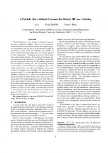
In each iteration, n particles are drawn from particle set Xt−1 and then propagated by means of a linear motion model as defined in Equation 8.   1 ∆t 0 i xti = 0 1 0 xt−1 + Nt (8) 0 0 1 with ∆t being the time interval between two subsequent sensor measurements, and Nt is a multivariate Gaussian random variable that models the system dynamics. New weights are derived by evaluating the propagated particles. For this purpose, the particle is projected onto the image plane of each camera. The pinhole camera model is used for this projection, as illustrated in Figure 1. Throughout this paper, the left camera will be the reference system. Given a point p in the left camera coordinate system, we can compute its position in the right one by p0 = R · p + t where t is a translation vector, and R is a rotation matrix. DOI: 10.1007/978-3-540-78157-8 http://www.springerlink.com/content/x80x381762364902/

(9)

G. Sommer and R. Klette (Eds.): RobVis 2008, LNCS 4931, pp. 327 – 340, 2008. c Springer-Verlag Berlin Heidelberg 2008

i

xt

yl

particle set

fl zl

i

u l ,t

Cl

yr

left camera

i

ur , t

xl fr right camera

image plane

Cr

zr

xr

Fig. 1. Top-down approach to 3D tracking. For evaluation, each particle xti is projected onto the image planes of the left and the right cameras.

The intrinsic parameters are the camera’s internal parameters specifying the way a three-dimensional point is projected onto the camera’s image plane. These parameters consists of the center of the camera image (u0 , v0 ) and the focal length f , i.e., the distance between the camera’s origin and its image plane. The image coordinates of the person’s head are calculated according to Equation 10 for both cameras. ux = − ppx ·z f + u0 uy =

py · f pz

+ v0

.

(10)

Furthermore, the radiuses of the projected sphere are determined. Now that the image coordinates of the person’s head uil,t and uir,t as well as the i and r i are known, the probability distributions p(L |xi ) and p(R |xi ) for radiuses rl,t t t t t r,t observing the person in the left and right image at the specified position xti is computed for each camera according to a color-based perception model that is introduced in the next section. After applying the model to both cameras, the new weights of the particles are calculated according to wti = p(Lt , Rt |xti ) = p(Lt |xti ) · p(Rt |xti ).

(11)

Here, for reasons of simplification, probabilistic independence is assumed between random variables Lt and Rt .

5

Color-Based Perception Model

The perception model proposed in this paper uses two kinds of information: Skin color is used as a global feature to track the person’s face and a histogram to describe the DOI: 10.1007/978-3-540-78157-8 http://www.springerlink.com/content/x80x381762364902/

G. Sommer and R. Klette (Eds.): RobVis 2008, LNCS 4931, pp. 327 – 340, 2008. c Springer-Verlag Berlin Heidelberg 2008

color distribution of the person’s upper part of the body used as local feature. This histogram not only specifies a distinct feature of the person, but is also independent of the person’s current orientation as long as parts of the person’s front are visible to the camera. Nonetheless, it has to be determined before tracking the person. A method to automatically initialize the tracker is described in Section 6. When doing color-based image processing, an appropriate color space has to be selected. By default, today’s cameras provide images in the RGB color space. But RGB has several disadvantages, for example, color information is not separated from luminance information. Therefore, RGB images are highly sensitive to varying lighting conditions and thus not adequate in this context. In the following the HSV color space has been chosen that represents color by the three components hue, saturation and value (sometimes also called intensity). Hue defines the actual color type (such as red, blue, green), saturation measures the intensity or purity of this color, and the value component expresses the brightness. 5.1

Color Histograms

Color histograms represent the color distributions of color samples C = {ci }i=1,...,nC in a discrete, non-parametric form. To achieve a certain tolerance for illumination changes, we separate color information (hue and saturation) from luminance information (value). The HS color space is partitioned into a number of equally sized bins with Nh bins for the hue component and Ns bins for the saturation component. These bins are populated using samples with sufficient color information, i.e. saturation and value larger than two predefined thresholds, see [5]. We use 0.1 and 0.2, respectively. Additionally, Nv bins are used for the value component of the remaining samples. The complete histogram consists of N = Nh · Ns + Nv bins. Each bin stores the number of times a color within its boundaries occurred in the color samples C. Given a color ci , the index of its associated bin is obtained by function b(ci ) ∈ {1, ..., N}. The histogram itself is defined as h = {qi }i=1,...,N

(12)

with nC

qi = α

∑ δ (i, b(c j ))

(13)

j=1

where α is a scaling factor, and δ (n, b(c j )) is the Kronecker delta function: ( 1, if i = j δ (i, j) = . 0, else 5.2

(14)

Skin Color Model

Skin color classification is one of the most widely used approaches for fast and easy identification of humans in color images. An overview of several methods for skin color DOI: 10.1007/978-3-540-78157-8 http://www.springerlink.com/content/x80x381762364902/

G. Sommer and R. Klette (Eds.): RobVis 2008, LNCS 4931, pp. 327 – 340, 2008. c Springer-Verlag Berlin Heidelberg 2008

modeling is given in [13]. In this paper, we want to model the distribution of skin color in the HSV space. Since only chromatic information is important for this task, the HS color space is used and illumination information, i.e., the value component, is not considered. As representation of this distribution we use a color histogram. The histogram hskin is populated with samples of skin color from several training images. Each bin stores the number of times a color within the bin’s boundaries occurred in the training samples according to Equation 13. Nskin The scaling factor α is set appropriately to ensure that ∑i=1 qskin,i = 1. So the histogram can be used as the discrete probability distribution p(St |xt ) for observing skin color at position xt : p(St |xt ) = qskin, j


with j = bskin I (ut )

(15)

where ut is the projected coordinate of xt in image I. 5.3

Histogram Tracking

The skin color model considers single pixels only. In addition, we use a color distribution model for image regions, i.e., a color histogram that represents the color distribution of a certain area of the person to be tracked. Here, the upper part of the person’s body is used as target model. Given the hypothetical person state x = (p, v, r)T as it is expressed by a particle, we use a quadratic image region R(x) with center c(x) and side length l(x): c(x) = (p0x , p0y + 2 · r0 )T l(x) = 2 · r0

(16)

where p0 is the image coordinate and r0 is the radius of the projected face for the current camera. A histogram with Nbody,h bins for hue, Nbody,s bins for saturation, and Nbody,v bins for the value component is used, Nbody = Nbody,h · Nbody,h + Nbody,h bins overall. A histogram generated for the quadratic image region R(x) is denoted as hbody (x). Again, the N

body histogram is normalized by the scaling factor α to ensure that ∑i=1 qbody,i (x) = 1. To measure the similarity between the target model and an candidate image region R(x) for the person’s body position, the Battacharyya distance is applied. The target histogram is denoted as h∗body = {q∗i } and has to be determined before the tracking process. An example of how to do this is given in Section 6. The distance between target and hypothetical body histogram is calculated as v u Nbody q u
∗ (17) D hbody , hbody (x) = t1 − ∑ q∗i qbody,i (x).

i=1

We now define the probability distribution p(Bt |xt ) as
 !  ∗ 1 D hbody , hbody (xt ) 2 p(Bt |xt ) = √ exp − . 2 σ 2πσ 2 1

DOI: 10.1007/978-3-540-78157-8 http://www.springerlink.com/content/x80x381762364902/

(18)

G. Sommer and R. Klette (Eds.): RobVis 2008, LNCS 4931, pp. 327 – 340, 2008. c Springer-Verlag Berlin Heidelberg 2008

Fig. 2. Two images that were simultaneously taken by the left and right camera to illustrate the person model. The upper rectangle shows the person’s face as it was detected in the user detection phase. The lower rectangle shows the part of the body that is used for tracking.

5.4

Particle Evaluation

Weights are assigned to each particle by evaluating the particle for each camera. The image coordinates uil,t and uir,t are calculated by projecting the particle xti onto the image i and r i . planes of the left and the right camera as well as the face radiuses rl,t r,t Afterwards, the skin color probabilities p(Sl,t |xti ) and p(Sr,t |xti ) are computed according to Equation 15 for both cameras. Furthermore, using Equation 18 the body color probabilities p(Bl,t |xti ) and p(Br,t |xti ) can be calculated. Again, for simplification, probabilistic independence between the random variables for skin color St and body color Bt is assumed. The resulting perception probability of each sample is given by p(zl,t |xti ) = p(Sl,t |xti ) · p(Bl,t |xti ).

(19)

The probability for the right camera is obtained analogous.

6

User Detection

The problem of the approach described so far is that the histogram used as target body model has to be initialized properly. We therefore propose a system working in two phases. In the user detection phase, the camera images are searched for the person that tries to interact with the system (this interaction can be started via the speech interface). When a person was detected in both camera images, a histogram of the person’s upper part of the body is initialized for each camera using the current image data. After the initialization the system switches into the user tracking phase, where the histogram is used as the target model to track the person via particle filtering. For user detection we have chosen a face recognizer based on the popular algorithm of Viola and Jones [10]. An implementation of which can be found in the OpenCV library [14]. Every time a user starts an interaction with the robot, the camera images are searched for frontal faces. DOI: 10.1007/978-3-540-78157-8 http://www.springerlink.com/content/x80x381762364902/

G. Sommer and R. Klette (Eds.): RobVis 2008, LNCS 4931, pp. 327 – 340, 2008. c Springer-Verlag Berlin Heidelberg 2008

We reduce the computational costs for face detection by first calculating regions of interest (ROIs) that limit the search space based on skin color. Therefor, each image is segmented into skin color regions and non-skin color regions. To achieve this, the probability p(S|u) of observing skin color is computed for each pixel u according to Equation 15. Those pixels whose probabilities are below a predefined threshold are set to 0, all other ones are set to 1. We use a threshold of 0.006. After that, skin clusters are calculated by region growing merging neighboring skin color pixels. For every cluster its enclosing bounding box is calculated. In a final step, boxes intersecting each other are further merged. We end up with distinct boxes that are used as the ROIs for the face detection algorithm. The face detector provides the coordinates ul and ur of the detected face as well as the side lengths sl and sr in the left and right image. To avoid the correspondence problem, i.e., determining which faces detected in both images belong to the same person, we assume that only one person is visible during the user detection phase. With coordinates and side length of the candidate face, we can calculate the position of the body area within the camera image according to Equation 16. The histograms of the regions in the left and the right camera image are calculated and used as the target body models h∗l,body and h∗r,body throughout the tracking phase. For initialization of the particles, the 3D position of the face is calculated via stereo triangulation. This is done by re-projecting the image points ul and ur into 3D, resulting in lines ll and lr with   (ul,x − u0 )/ f (20) ll (λ ) = λ (ul,y − v0 )/ f  1 and 

 (ur,x − u0 )/ f lr (λ ) = λ · R−1 (ur,y − v0 )/ f  − t 1

(21)

where R and t are the extrinsic parameters of the right camera. The 3D coordinates can now be determined by calculating the intersection between both lines. Since lines ll and lr may not intersect due to measurement errors, the problem is solved using a least square method that determines the λ = (λl , λr )T that minimizes
2 ε = ll (λl ) − lr (λr ) .

(22)

The calculated 3D position x f = ll (λl ) of the face is now used to initialize the particles of our tracker according to  i   p0 xf x0i =  vi0  =  0  + Nσ (23) 0 r0i where N is a Gaussian multivariate with a mean value of 0 and variance σ . Furthermore, the weight of each particle is calculated as DOI: 10.1007/978-3-540-78157-8 http://www.springerlink.com/content/x80x381762364902/

G. Sommer and R. Klette (Eds.): RobVis 2008, LNCS 4931, pp. 327 – 340, 2008. c Springer-Verlag Berlin Heidelberg 2008

wi0 = √

  1  d(x f , x0i ) 2 exp − 2 σ 2πσ 2 1

(24)

where d(x f , x0i ) is the distance between both vectors.

7

Experiments

The proposed person tracker has been implemented in C++ and tested on a laptop with a 1.99 GHz Pentium 4 processor and 1GB memory. Two FireWire web cameras with a maximum frame rate of 15 fps were mounted with a distance of 20 cm between each other. The cameras were calibrated according to the method described in [15]. Training of the skin color classifier was done with 80 training images from the Internet and databases showing persons from different ethnic groups. All samples were converted into the HS color space and sampled into a histogram with 30 × 32 bins. No samples of persons appearing in the experiments where part of the training set. Histograms with 30 × 32 × 10 bins were used for body tracking. The variance in Equation 18 was set to 0.12. The Gaussian random variables used in Equation 8 were set to 0.96 m for position, 1.44 ms for velocity, and 0.48 m for scale error of the head radius. The particle filter itself worked with 400 particles. Every time the effective number of particles Ne f f was smaller than 100 resampling was performed. The system has been applied to a variety of scenarios. In each test run, the tracker was automatically initialized as described in Section 6. The system worked with 12 to 15 fps, thus achieving real-time capabilities. Several test runs were used to compare the proposed method with a classical bottomup method where face detection was performed in every image and the 3D position was determined via stereo triangulation. The resulting position was compared to the mean state of the particle set of our approach that is calculated as n

E[Xt ] = ∑ wti · xti .

(25)

i=1

Results from one training sequence can be seen in Figure 4 and are summarized in Table 1. Figure 3 shows the trajectories generated by both methods. The path produced by the bottom-up approach has many leaps since face detection is erroneous and no additional smoothing filter, such as a Kalman filter. In Figure 3(b) the data from stereo triangulation was additionally approximated with a Bezier curve resulting in a curve comparable to the one produced by our technique. Table 1. Comparison of bottom-up and proposed top-down approach.

XZ plane Y-axis

Mean distance [cm] Standard deviation [cm] 12.39 8.81 1.32 0.92

DOI: 10.1007/978-3-540-78157-8 http://www.springerlink.com/content/x80x381762364902/

G. Sommer and R. Klette (Eds.): RobVis 2008, LNCS 4931, pp. 327 – 340, 2008. c Springer-Verlag Berlin Heidelberg 2008

-350 #50

bottom-up smoothed bottom-up top-down

bottom-up top-down

#56

y [cm]

#56

-300

#54

200

#50

150

#12 z [cm]

100 50 0

-250 #54 #12

-300

80

-200

60

-250 20

-200 z [cm]

-20

-150

-40

40

0 x [cm]

-150 -60

-40

-20

0

20

40

60

80

x [cm]

(a)

(b)

Fig. 3. Trajectories produced by stereo triangulation (dashed lines) and proposed approach (solid lines). Images associated to marked positions are shown in Figure 4

Figure 5 show a second test sequence in which the user’s face is temporarily and partially occluded. As can be seen, the system manages to track the person if the face is occluded or if the person is looking into a different direction.

8

Conclusion

In this paper, we have presented a method for tracking a person in 3D with two cameras. This tracker was designed for robots, so different constraints had to be considered. Since robots work in highly dynamic environments a probabilistic approach has been chosen. Furthermore, a problem of real-world trackers is that users are often temporary or partially occluded. That is why a top-down approach based on a particle filter was selected. In this framework, particles represent hypotheses for the person’s current state in the world coordinate system. The particles are projected onto the image planes of both cameras, and then evaluated by a color-based perception model. Our model uses skin color cues for face tracking and color histograms for body tracking. We also provided a method to initialize the tracker automatically. We showed that our system tracks a person in real time. The system also manages to track a person even if it is partially occluded, or if the person is looking away from the cameras. In the future, we plan to use the proposed system on a mobile robot. For this purpose, we want to determine the robot’s motion via image-based ego-motion estimation.

References 1. Thrun, S.: Probabilistic Algorithms in Robotics. AI Magazine 21(4) (2000) 93–109 2. Gorodnichy, D.O.: On Importance of Nose for Face Tracking. In: Proceedings of the Fifth IEEE International Conference on Automatic Face and Gesture Recognition, Washington, DC, USA, IEEE Computer Society (2002) 188

DOI: 10.1007/978-3-540-78157-8 http://www.springerlink.com/content/x80x381762364902/

G. Sommer and R. Klette (Eds.): RobVis 2008, LNCS 4931, pp. 327 – 340, 2008. c Springer-Verlag Berlin Heidelberg 2008

3. Raja, Y., McKenna, S., Gong, S.: Segmentation and Tracking using Colour Mixture Models. In: Proceedings of the Third Asian Conference on Computer Vision. (1998) 607–614 4. McKenna, S., Raja, Y., Gong, S.: Tracking Colour Objects using Adaptive Mixture Models. IVC 17(3/4) (March 1999) 225–231 5. P´erez, P., Hue, C., Vermaak, J., Gangnet, M.: Color-Based Probabilistic Tracking. In: Proceedings of the 7th European Conference on Computer Vision-Part I, London, UK, SpringerVerlag (2002) 661–675 6. Focken, D., Stiefelhagen, R.: Towards Vision-Based 3-D People Tracking in a Smart Room. In: Proceedings of the 4th IEEE International Conference on Multimodal Interfaces (ICMI 2002). (2002) 400–405 7. Gorodnichy, D., Malik, S., Roth, G.: Affordable 3D Face Tracking using Projective Vision. In: Proceedings of International Conference on Vision Interface (VI’2002). (2002) 383–390 8. Kobayashi, Y., Sugimura, D., Hirasawa, K., Suzuki, N., Kage, H., Sato, Y., Sugimoto, A.: 3D Head Tracking using the Particle Filter with Cascaded Classifiers. In: BMVC06 - The 17th British Machine Vision Conference. (2006) I:37 9. Nickel, K., Gehrig, T., Stiefelhagen, R., McDonough, J.: A Joint Particle Filter for Audiovisual Speaker Tracking. In: Proceedings of the 7th International Conference on Multimodal Interfaces, New York, NY, USA, ACM Press (2005) 61–68 10. Viola, P., Jones, M.: Rapid Object Detection using a Boosted Cascade of Simple Features. In: Proceedings IEEE Conf. on Computer Vision and Pattern Recognition. (2001) 11. Isard, M., Blake, A.: CONDENSATION – Conditional Density Propagation for Visual Tracking. International Journal of Computer Vision 29(1) (1998) 5–28 12. Liu, J., Chen, R.: Sequential Monte Carlo Methods for Dynamic Systems. Journal of the American Statistical Association 93(443) (1998) 1032–1044 13. Kakumanu, P., Makrogiannis, S., Bourbakis, N.: A Survey of Skin-Color Modeling and Detection Methods. Pattern Recognition 40(3) (2007) 1106–1122 14. OpenCV-Homepage: http://sourceforge.net/projects/opencvlibrary/. 15. Zhang, Z.: Flexible Camera Calibration by Viewing a Plane from Unknown Orientations. In: Proceedings of the International Conference on Computer Vision. (1999) 666–673

DOI: 10.1007/978-3-540-78157-8 http://www.springerlink.com/content/x80x381762364902/

G. Sommer and R. Klette (Eds.): RobVis 2008, LNCS 4931, pp. 327 – 340, 2008. c Springer-Verlag Berlin Heidelberg 2008

(a) Frame 12

(b) Frame 50

(c) Frame 54

(d) Frame 56

Fig. 4. Sequence to compare bottom-up tracking (solid lines) with the approach described in this paper (dashed lines). Bellow each image pair the room is shown in bird’s eye view with marks of the head position calculated by bottom-up (red circle), particles (marked as x) and mean state of top down approach (black circle).

DOI: 10.1007/978-3-540-78157-8 http://www.springerlink.com/content/x80x381762364902/

G. Sommer and R. Klette (Eds.): RobVis 2008, LNCS 4931, pp. 327 – 340, 2008. c Springer-Verlag Berlin Heidelberg 2008

(a) Frame 26

(b) Frame 34

(c) Frame 56

(d) Frame 66

(e) Frame 100

(f) Frame 105

10.1007/978-3-540-78157-8 Fig. 5. TestDOI: sequence that shows the robustness to occlusion. http://www.springerlink.com/content/x80x381762364902/