3D-Ultrasonic Source Localization System Design ...

Final Report : 3D-Ultrasonic Source Localization System Design using Time Difference of Arrival base on GCC Method Bima Sahbani#1 , Panji Ramadhan*2 , Monang Kevin#3 1,2,3

Electrical Engineering Department - School of Electrical Engineering and Informatics, Bandung Institute of Technology Ganesa St No.10, Bandung, West Java [email protected] [email protected] 3

[email protected]

Abstract— This paper explains a project of sound localization implementation using VLS I system design base on verilog structural programming language. 3-D Ultrasonic S ound localization is used to automatically identify and track the location of objects or people by his sound in real time, usually within a building or other contained area. This project is about building the sound localization chip design in FPGA with verilog. This chip can detect and locating ultrasonic source. Ultrasonic is sound with a frequency greater than the upper limit of human hearing (greater than 20 kHz). S ystem will be implemented by some modular VLS I design, Including hardware Configuration consist of Analog IC modelling which includes Heterodyning and S ignal Filtering, Digital S ignal Processing by using ADC 10 bit, digital Filtering using FIR Generalized Cross Corelation (GCC) to determine time difference among array of microphone. And Triangulation algorithm as the main localization algorithm. In the hardware configuration and localization algorithm. Keywords—S ound S ource Localization, TDOA, GCC, Ultrasonic.

I. INT RODUCT ION 3-D Sound localization is used to automatically identify and track the location of objects or people by his sound in real time, usually within a building or other contained area. Examples of real-time sound localization include sound tracking for humanoid robot, locating of sniper position in war tech nology, etc. Two important points to be considered when developing such kind of device are its physical dimensions and response speed. A common approach for sound localization is the use of microphone array. This method will give us a good precision result. But it usually get an expensive price to be built even if we use Digital Signal Processor (DSP) such. It also require a large amount of power. For example, the Huge Microphone Array system developed by Brown University which use multiple DSP processors and buffers for sound localizatio n with an average power consumption of 400mW per microphone. This will be so difficult to be implemented in

mobile phone or other device that generate not much power. To overcome this kind of problem, we must use the method that is less power, less expensive, and smaller than sound localization using digital signal processor. So the best answer containing those criteria is custom-designed VLSI chip. On this project, we will implement chip design in Field Programmable Gate Array (FPGA) with verilog. II. OBJECT IVE AND PROBLEM LIMIT AT ION This project is about building the sound localization chip design in FPGA with verilog. This chip can detect and locating ultrasonic source. Ultrasonic is sound with a frequency greater than the upper limit of human hearing (greater than 20 kHz). This project is focusing for detecting and locating animal that use ultrasound as their navigation tool such as bat. Bats use ultrasound ranging from 16 kHz to 120 kHz for their navigation. This project can detect ultrasound frequency ranging from 15-40 kHz. Output of the system is position point of sound source in cartesian coordinate (x, y, z). . III. THEORET ICAL A PPROACH A. General Cross Correlation for Computing TDOA There are so many sound localization method created in research such as Pulsed Neural Network, etc. But the most common method is to estimate the time delay of arrivals (TDOA) between all microphone pairs. To get the value of TDOA, we use generalized cross correlation (GCC) because GCC method is relatively simpler and more efficient than the other method. We assume that there are two microphones which receive the signals 𝑚1 (𝑡) and 𝑚2 (𝑡) respectively. These signals include noise, reverberation, and a time-delayed, 𝜏 (with TDOA version) of a speech signal, will be analyzed in order to get 𝜏 or

TDOA parameter. Mathematical model of GCC method to compute TDOA is defined below: 𝜏̅ = arg max ∫ 𝑊 (𝜔 ) 𝑀1 (𝜔) 𝑀2 (𝜔 ) 𝑒 −𝑗𝜔𝛽 𝑑𝜔

(1)

𝛽

where 𝜏̅ is an estimate value of 𝜏, 𝑀1 (𝜔) and 𝑀2 (𝜔 ) are the Fourier transforms of the first and second microphone signals, respectively, and 𝑊 (𝜔) is a cross correlation weighting function. Two different choices for 𝑊 (𝜔 ) include : 𝑊𝑝𝐻𝐴𝑇 (𝜔) =

1 |𝑀1 (𝜔) ||𝑀2 (𝜔) |

(2)

(3)

𝑊𝑈𝐶𝐶 (𝜔) = 1

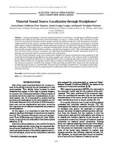
Figure 3.1. The array with four microphones

Microphone m1 is chosen to be the reference microphone. The geometry relationship can be written as : (5)

The PHAT weights correspond to the PHAse Transform, and are known to be effective in reverberant environments. The UCC weights correspond to the Unfiltered Cross Correlatio n technique, which is simply a standard cross correlation without any weights. The single-segment GCC for discrete-time signals can alternatively be expressed as:

where j = 2, 3, 4, is the TDOA between mj and m1 . If is positive, mj is farther to sound source than m1 , and negative means mj is nearer to sound source. And c is the sound speed, which is considered as a constant. Eq. (5) can be rewritten as (6)

𝑁 /2

𝜏̅ = arg max ∑ 𝑊(𝑘) |𝑀1 (𝑘) | | 𝑀2 (𝑘) |cos (θ(k) ) 𝛽

(4)

𝑘=0

(7)

where θ (k) = ∠𝑀1 (𝑘) − ∠𝑀1 (𝑘) − 2𝜋 𝐹𝑠 𝑘𝛽/𝑁 is defined as the phase error, k is the index of the discrete fourier transforms (or, alternatively, the fast fourier transforms (FFTs)) of the signals involved, 𝑁 is the total number of samples in each segment, and 𝐹𝑠 is the sampling frequency. Equation 4 can be viewed as a weighted rewardpunish function of the phase error at different frequencies. Ideally, the phase error would be close to zero, resulting in the maximization of equation 4. The cosine phase error selector function in effect rewards lower phase errors and punishes higher phase errors. B. Triangulation Microphones

The square of Eq. (2) can be written as

Method Using An Array

with

where: (8) Eq. (9) can be obtained deriving from Eq. (7) :

(9)

Four

The array is positioned in the x-y plane, with an X shape, as shown in Fig. 1. The micro-phones are numbered as 1 to 4. The microphone mi (i =1~4) is located at a fixed position, with coordinate (xi, yi, 0). The sound source is located at arbitrary point in the space, with coordinate (xs, ys, zs). (i =1~4) and represents the vector from the origin to microphones or the sound source.

IV. SYST EM SPECIFICAT ION AND DESIGN Where

(10)

The estimation of coordinates of sound source is presented as Eq. (9). As the z-coordinate is square root of a function, it

has two solutions, one positive and the other negative. In a practical application, the sign of z-coordinate is predefined, so that the z-coordinate is certain.

IV. FINAL SYST EM DESCRIPT ION After doing design iteration and optimization the final system can be divided nto 2 part implementation 1. Analog IC modelling for analog Signal Conditioning ADC

mixer

S1

D

S2

EN

+

C1 C2 B

Low Pass Filter

Digital Signal

ADC

microphone

mixer

S1

D

S2

EN

+ Multiplexer

C1 C2 B Output Cordic channel1

Low Pass Filter Heterodyne Signal 40KHz

amplification, bandpass filtering, and then sampling at 90 KHz with 8 bits per sample. The 8 most significant bits of the samples are then fed digitally to a Altera DE2 Board FPGA , where the TDOA computation takes place. The buffers were then windowed using Hamming windows, converted to 16 hit floating point representations, and stored in two Fast Fourier Transform (FFT) buffers, as shown in Figure 4.2.The FFT is performed in-place on each of the buffers. The CORDIC algorithm is utilized to calculate the Fourier Transform sines and cosines and to convert complex numbers from real-imaginary to magnitude-phase representations. The CORDIC algorithm was chosen since it can perfor m magnitude-phase estimation quickly without significant hardware requirements.

CHANNEL1 GCC 1

S1

D

FS S4 CHANNEL1 GCC2

CHANNEL1 GCC3 C1

Figure 4.1. Analog IC schematics modelling for Supply 4 Input audio signal (array of Microphone)

C2

ENB

GCC

TDOA Output

Multiplexer

Ultrasonic audio signal that we will detect in the system is specified into 40KHz Frequency, Base on the Nyquist Criterio n minimum Sampling frequency should twice from the targeted signal, in other word The more ADC clock so the more Power need for This subsystem because of that. There will be add ed heterodyne unit to shift frequency range of the audio signal. This unit beside to limit sampling clock also to reduce noise as known that noise intensity in high frequency domain usually higher than the lower one. The Analog IC is modelled by using Matlab code on the appendixes. Input audio signal is got by Ultrasonic Transducer diameter 13mm. This transducer will transfer audio signal to the computer via serial arduino. Than Matlab program will return heterodyned and filtered digital signal [10bits data] to the FPGA via another serial. Beside the data flow of the signal, another crucial thing is the location of Microphone array. For Triangulation algorith m we’ve changed Microphone array configuration fro m tetrahedral to planar This configuration likely simpler than the initial one (tetrahedral configuration).

2.

4

VLSI Modular system Design for Sound Localizatio n algorithm as Digital IC design. The proposed TDOA estimation technique is employed for single microphones. Each microphone undergoes

CHANNEL2 GCC 1

S1

D

S4 CHANNEL2 GCC2

Output Cordic channel2

CHANNEL2 GCC3

C1

C2

ENB

Figure 4.2 TDOA module schematics

Once the magnitude and phases of each of the two channels are calculated, the modified GCC technique of equation 5 is used to obtain a TDOA estimate, as shown in Figure 4.3. This TDOA estimation involves searching for the GCC maximizin g T according to equation 5. The search step size started at -30TS and ended at 30TS in TS step sizes, where Ts = 1/FS is the sampling period. Also, a value of 0.5 radians was used for e. The hardware implementation utilizes a 3-stage pipeline architecture in order to obtain real-time TDOA estimates. The first stage consists of acquiring the input samples, the second stage consists of FFT computation and conversion to magnitude-phase representation, and the final stage consists of TDOA estimation. While two GCC buffers are sufficient, three buffers are used in order to keep the results of the previous time segment. This allows for temporal smoothing which results in more accurate localizations. Time difference of Arival method generally just return the time difference value, bu for localization process, there will be needed Triangulation algorithm to represent time difference

into Space representation. On this paper localization algorith m using Triangulation algorithm to determine x-y-z space representation. Then this coordinate will be represented to the spherical room coordinate system using transformation. Or this system can be described in the block diagram in figure 4.4 below. Microphone 1

a. Audio signal Generating in 44 KHz. From this procedure there will be got the result below

Microphone 2 TDOA

TDOA

Microphone 2

Microphone 3

Microphone 1

Microphone 2 TDOA

TDOA

t Microphone 3

Spherical Coordinate System

Microphone 4

Microphone 1

Microphone 3 TDOA

TDOA

Microphone 4

Room Transformation

Microphone 4

X,y,z representation

TRIANGULATION

Figure 5-1 44KHz Audio signal

Figure 4.4 Localization algorithm using Triangulation

V. SYNT HESIS AND PART TEST ING Implementation process that have be done is including system part Synthesizing and Testing. Because of the final system is consist of 2 subsystem (Analog IC modelling and FPGA based Sound source localization). 1. Synthesizing Analog IC modelling For this synthesizing Process there will be conducted some testing methode particullarly in frequency Domain. The testting steps including

Figure 5-2 Signal Spectrum

c. b.

Testing Heterodyning Process.

Signal Digitizing (10 bits) and Filtering using FIR (Finite Impulse Response Filter)

Figure 5-3. Inphasa Heterodyne Figure 5-5. 10 bit level ADC Result

Figure 5-4. Quadrature Heterodyne Figure 5.6. Digital Signal Spectrum

TDOA result and Sign (+/-)

Figure 5-7. Digital Filter Result

Figure 5-9 Filtered Digitized signal

This testing is done using Matlab resulting Digitized signal, and by adjusting the delay order of the sampled signal. 3.

Synthesizing Triangulation Part to generate Sound Source 3D coordinate from TDOA data

This Component also has been successfully synthesized by data from TDOA, It has been implemented the triangulation algorithm there will be return x, y, and z2 coordinate value.

Figure 5-8 Filtered Digitized signal

By the result above there will be known that the system working properly in modelling analog IC 2.

Synthesizing GCC algorithm to generate TDOA.

This Component was successfully being synthesize and testing using Dummy data by delaying identical array of digital signal in table below and the testing result can be shown as the figure below.

Estimated x Estimated y Estimated z2 Figure 5-9 Filtered Digitized signal

But this Implementation still have a defect in detecting impossible condition of TDOA, particularly for the sign case of each tdoa (∆𝑡1,2; ∆𝑡1,3;; ∆𝑡1,4) This condition will be handled by negative z 2.

REFERENCES [1]

VI. NEXT W ORK For the next work, there will be part integration and Hardware Implementation using real circuit analog IC and Ultrasonic Transducer. There will be need ADC component from another embedded system like Arduino.

VII.

[2]

[3]

CONCLUSIONS [4]

Each part of the system successfully tested in the simulation on PC. And for the next work each part will be integrated to the one system and be going to be implemented in FPGA DE1.

[5] [6]

D.Nguyen, P. Aarabi, and A. Sheikholeslami. Real-time Sound Localization Using Field-Programmable Gate Arrays. In The Edward S. Rogers Sr. Department of Electrical and Computer Engineer, University of Toronto. Feng M io, Yang Diange, 2014, “A Triangulation M ethod base on the Phase Difference of Arrival Estimation For Sound Localization”, ICSV21-Beijing, RRC. Jean-M arc Valin, Franc¸ ois M ichaud, Jean Rouat, Dominic Letourneau. Robust Sound Source Localization Using a M icrophone Array on a M obile Robot. In Research Laboratory on Mobile Robotics and Intelligent Systems Department of Electrical Engineering and Computer Engineering Universite´ de Sherbrooke. Kim, Yong Eun, Dong Hyun Su, “Sound Source Localization Method using Region Selection”, Korean Automitive Technology Institute-Republik Korea. “Sonar”, Columbia Electronic Encyclopedia, 6th Edition. 2000, Columbia University Press-USA http://www.kayelaby.npl.co.uk/general_physics/2_4/2_4_1.htm l [accesed on October 10th 2015; 11:30 am]

Appendixe Sampling using Analog IC Modeling % Module IC analog Modeling %The main goal of This module is to make analog IC modeling until %Analog to Digital Converter which will supply digital data for determine %sound source coordinate %generate signal Ultrasonic frameSize = 2047; inFs = 90e3; sigfreq = 44e3; hchirp = dsp.Chirp(... ‘SweepDirection’, ‘Bidirectional’, ... ‘TargetFrequency’, sigfreq, ... ‘InitialFrequency’, 0,... ‘TargetTime’, 1, ... ‘SweepTime’, 1, ... ‘SamplesPerFrame’, frameSize, ... ‘SampleRate’, inFs); for k = 1:frameSize % Source sig = step(hchirp); end f1 = figure; plot(step(hchirp)); title(‘ULTRASONIC 44KHz SIGNAL’); %validation %fft for spectrum form confirmation Fs = 180e3; % Sampling frequency T = 1/Fs; % Sample time L = frameSize; % Length of signal t = (0:L-1)*T; % Time vector NFFT = 2^nextpow2(L); % Next power of 2 from length of y Y = fft(sig,NFFT)/L; f = Fs/2*linspace(0,1,NFFT/2+1); f2=figure; plot(f,2*abs(Y(1:NFFT/2+1))); title(‘Single-Sided Amplitude Spectrum of y(t)’); xlabel(‘Frequency (Hz)’); ylabel(‘|Y(f)|’); %Heterodyning freqheter = 40e3; sigmixq = sin(2*pi*freqheter*t); sigmixi = cos(2*pi*freqheter*t); sigheterq = 2*(sig.*transpose(sigmixq)); sigheteri = 2*(sig.*transpose(sigmixi)); sigheter = sigheterq + sigheteri; f3=figure; shq = fft(sigheterq,NFFT)/L; f = Fs/2*linspace(0,1,NFFT/2+1); plot(f,2*abs(shq(1:NFFT/2+1)));

title('Single-Sided Amplitude Spectrum of yq(t)'); xlabel('Frequency (Hz)'); ylabel('|Y(f)|'); f4=figure; shi = fft(sigheteri,NFFT)/L; f = Fs/2*linspace(0,1,NFFT/2+1); plot(f,2*abs(shi(1:NFFT/2+1))); title('Single-Sided Amplitude Spectrum of yi(t)'); xlabel('Frequency (Hz)'); ylabel('|Y(f)|'); f5=figure; sh = fft(sigheter,NFFT)/L; f = Fs/2*linspace(0,1,NFFT/2+1); plot(f,2*abs(sh(1:NFFT/2+1))); title('Single-Sided Amplitude Spectrum of yi(t)'); xlabel('Frequency (Hz)'); ylabel('|Y(f)|'); %ADC MAXVAL = max(sigheter);%get maxval==2.8162 MINVAL = min(sigheter);%get minval==-2.8175 DigSig = (sigheter+2.8175)*181.72;%181.72 = 1024/(2*2.8175) f6=figure; n=1:2047; plot(n,DigSig); title('DIGITAL SIGNAL'); xlabel('SAMPLE'); ylabel('SIGNAL'); f7=figure; DS = fft(DigSig,NFFT)/L; f = (2)/2*linspace(0,1,NFFT/2+1); plot(f,abs(DS(1:NFFT/2+1))); title('spektrum digital signal'); xlabel('Frequency (pi)'); ylabel('|Y(omega)|'); %Digital Filtering FIR Fc = 0.15; N = 2047; d=fdesign.lowpass('Fp,Fst,Ap,Ast',0.15,0.2,1,400); Hd = design(d,'equiripple'); filtsig = filter(Hd,DigSig); f8=figure; DS = fft(filtsig,NFFT)/L; f = (2)/2*linspace(0,1,NFFT/2+1); plot(f,abs(DS(1:NFFT/2+1))); title('spektrum digital signal after filtering'); xlabel('Frequency (pi)'); ylabel('|Y(omega)|'); f9=figure; n=1:2047;

plot(n,filtsig); title('Filtered Signal'); xlabel('SAMPLE'); ylabel('SIGNAL'); %digitized signal finalresult=zeros(frameSize,1); for k = 1:frameSize if(filtsig(k) > 0.000)finalresult(k) =uint16(filtsig(k)); else finalresult(k) = 0; end end f10=figure; n=1:2047; plot(n,finalresult); title('Digital Filtered Signal'); xlabel('SAMPLE'); ylabel('SIGNAL');

TDOA generating using GCC algorithm // Module GCC : for measuring tdoa module gcc(clk,rst,en,tdoa); parameter N=2048; // Number of samples parameter idle=0; parameter cross_cor=1;// crosscorrelation parameter adj_arg=2; parameter arg_max=3; //finding the max value of crosscorrelation // Input - output input clk,rst,en; output [15:0]tdoa; reg reg reg reg reg reg reg

[9:0]m1a[0:N-1]; [9:0]m1[0:3*N-1]; [9:0]m2[0:N-1]; [1:0]state; [31:0]cc[0:2*N-1][0:N-1]; [15:0]tdoa_adj[0:2*N-1][0:2*N-1]; [15:0]tdoa1;

// Counter reg [15:0] reg [15:0] reg [15:0] reg [15:0] reg [15:0] reg [15:0] reg [15:0]

c0; c1; c2; c3; c4; c5; c6;

wire [1:0]nstate; // input data to memory initial begin $readmemh ("M1.list",m1a);

$readmemh ("M2.list",m2); end // reset adjusting always @(posedge clk) begin if (!rst) state >7)/a12; assign sye = sab^sa12; endmodule // Module to calculate h1-h2 module diff (h1,h2,sh1,sh2,r,sr); input [31:0] h1; input [31:0] h2; input sh1,sh2; output [31:0] r; output sr; wire [31:0] r1; wire [31:0] r2; wire [31:0] r3; assign r1 = h1-h2; assign r2 = h2-h1; assign r3 = h2+h1; assign r = (!(sh1^sh2))&&(h1>=h2) ?r1: (!(sh1^sh2))&&(h1h2) ?0: (sh1==0&&sh2==0)&&(h1h2) (sh1==1&&sh2==0)&&(h1h2) (sh1==0&&sh2==1)&&(h1h2) 0;

?1: ?1: ?0: ?0: ?1:

endmodule module count_a1s(t12,t13,s12,s13,a1,sa1); parameter x1 = 10; parameter x2 = 20; parameter x3 = 10; parameter x4 = 20; parameter y1 = 10; parameter y2 = 20; parameter y3 = 10; parameter y4 = 20; input [31:0] t12; //value of t12 input [31:0] t13; //value of t13 input s12,s13; //sign of t12 and t13 output [31:0]a1; //value of a1 output sa1; //sign of a1 wire wire wire wire wire wire wire wire

[31:0] xt12; [31:0] xt13; [31:0] yt12; [31:0] yt13; sxt12,sxt13,syt12,syt13; [31:0] num; [31:0] den; snum,sden;

assign assign assign assign

xt12 = (x1+x3)*t12; xt13 = (x1+x2)*t13; sxt12 = s12; sxt13 = s13;

assign assign assign assign

yt13 = (y2-y1)*t13; yt12 = (y1+y3)*t12; syt13 = !s13; syt12 = s12;

diff diff_num_a1(xt12,xt13,sxt12,sxt13,num,snum); diff diff_den_a1(yt13,yt12,syt13,syt12,den,sden); assign a1 = (num