VLSI Design for 3D-Ultrasonic Source Localization using General Cross Correlation and Triangulation Algorithm Bima Sahbani1, Panji Ramadhan2, Monang Kevin Napitupulu3 1, 2, 3
Electrical Engineering Department, ITB Jalan Ganesa No 10 Bandung, Indonesia 1
[email protected],
[email protected],3
[email protected]
Abstract—Localization system is part of the study in navigation. One of the most navigation systems which are relatively robust in many propagation media and accommodates inaudible sound is Ultrasonic wave. But ultrasonic wave works in the high-frequency domain so that there will need special treatment for implementation in the navigation system. In this paper, there will be explained VLSI system modeling that accommodates ultrasonic sound localization. Under this research, ultrasonic localizer system is implemented in two basic subsystems, the first is signal conditioning using heterodyne and low pass filter. Then, after the signal has been digitized, it will be processed in Digital signal processor under General Cross Correlation (GCC) and triangulation algorithm to get the final result that represents 3D Cartesian coordinate. The result of this research is 3D ultrasonic localizer has been brought to be successfully implemented in model simulation using Modelsim® and Matlab®. The system has been tested and compared with theoretical computation. For the future implementation, the signal conditioning system is potentially implemented in analog IC Design. Keywords— Ultrasonic Localization; 3D Cartesian Coordinates; Triangulation; General Cross Correlation; Heterodyning Filter.
I. INTRODUCTION Nowadays, Navigation system is one of the most urgent systems in many purposes especially in transportation, military, robotics even more in industry. The most common medium for the navigation system is the mechanical and acoustic wave. Acoustic wave based navigation has good performance in accuracy and usually more robust to be used in another transferred medium especially in solid and liquid. But human ability to hear acoustics wave in certain frequency make a big trouble to be used. Ultrasonic wave is kind of acoustic wave. This wave has the high-frequency domain, high energy level, wide range transport and usually more robust in the liquid medium. The most important thing from ultrasonic that its frequency domain is far from human audible sound. This condition will be such beneficial that can be implemented for multipurpose navigation. But the most trade-off for the system to process ultrasonic-based system comes from its frequency, there will need the system which could accommodate high-frequency processing or the most visible treatment is signal conditioning before work in the digital domain. To overcome this problem, we must use the method that is less power, less expensive, and smaller than sound localization using a digital signal processor. So the best answer containing those criteria is custom-designed VLSI chip.
Various research about sound source localization has been conducted in some developing method in satisfying system performance including minimizing localization error [9], system robustness by developing the physical configuration of microphone arrays [3]. These all developing methods are generally used to make sound source localization could be implemented in multipurpose need. By then, most of the research accommodates algorithm development such that there still the lack of analog approach modeling for signal conditioning in the localization system. Whereas by this approach there will be potentially brought the system into more flexible especially in the frequency range for multipurpose, and multi-spectra sound localization. From this state of the art, this research is conducted to stimulate analog signal conditioning approach for sound localization. By this paper, there will be explained about our research that brings the VLSI system model which is integrated with signal conditioning system modeling for localizing ultrasonic wave in 3D Cartesian coordinate. This research is done by considering some problem limitation for indoor implementation, short range localization. This paper has 6 main points including, problem limitation in section 2, section 3 will explain the basic theory which is used for the system implementation, system design in section 4, Testing and simulation in section 5, and the 6th section explains the potential future research from the implementation point of view. The digital domain processing will be done using Verilog language for VLSI system design, in the other side the signal conditioning will be modeled using Matlab®. II. OBJECTIVE AND PROBLEM LIMITATION This project is about building the sound localization chip design in FPGA using Verilog. This chip can detect and locate the ultrasonic source. Ultrasonic is sound with a frequency greater than the upper limit of human audible sound (greater than 20 kHz). This project is focusing for detecting and locating the animal that uses ultrasound as their navigation tool such as the bat. Bats use ultrasound ranging from 16 kHz to 120 kHz for the navigation. By this project, it was expected that the system can detect ultrasound frequency in the range from 15 to 40 kHz. The output of the system is position point of ultrasonic source in the 3 Dimension-Cartesian coordinate (x, y, z). We also assumed that the system accommodates unidirectional Ultrasonic sensor, such that the planar configuration is the most visible in use.
III. FUNDAMENTAL THEORY
𝑇(𝑧) =
A. Introduction to High Frequency Signal Conditioning Heterodyne Method In high-frequency domain signaling, there had been a trouble in sampling and analyzing the signal from its disturbance noise. The simplest solution for this problem is to deliver the signal into more visible frequency domain then the signal will simply be filtered inside the desirable frequency range. This technique actually is based on the radio modulation-demodulation techniques. One of the most common methods is signal heterodyning [6]. Heterodyning method principally comes from sinusoidal multiplication that potentially brings the signal to certain frequency shifting that could be described in the equation below. 1 sin(𝑎𝑡) cos(𝑏𝑡) = (cos((𝑎 + 𝑏)𝑡) + cos((𝑎 − 𝑏)𝑡)) 2
(1)
Coincidentally, if two sinusoidal-based signals are multiplied each other, then the signal will be shifted in the frequency domain as much as the multiplicand signal frequency so that from this simple principle there will be defined certain frequency range shifting. The most visible modeling for this signal conditioning principle is using the mixer. B. Introduction to Signal Filtering [6] It was common sense that one of the performance indicators of signal processing is noise cancellation. There are many kinds of method for noise cancellation, oversampling, filtering and semantic approach. The most common and easiest method is signal filtering. There are many kinds of signal filtering base on the frequency range, they are Low Pass Filter (LPF), Band Pass Filter (BPF), High Pas Filter (HPF), and Notch Filter. Moreover in the approach of the method, Chebyshev, Hamming, and Butterworth is the most common method.
𝑌(𝑧) = 𝐻(𝑧𝑒 +𝑗𝜔ℎ 𝑡 )𝐻(𝑧𝑒 −𝑗𝜔ℎ 𝑡 ) 𝑋(𝑧)
In the circuit s shown above, the three complex heterodyne operations have the effect of rotating poles and zeros of the fixed coefficient filters H(z), first to the left, then twice to the right, and finally, once to the left much like opening a combination lock. The effect is to generate a new transfer function T(z), which shifts the notch or band-pass frequency to a new location specified by the heterodyne frequency Wh. D. Introduction to Generalized Cross Correlation in TDOA Generating [1][2][10] In many signal-localization algorithms, there will be need comparable parameter that could be used consideration to the signal source transfer from the environment to the specific sensor. This condition also occurs for sound source localization. The most visible comparable parameter in sound source localization is the time difference of sound’s arrival among the sensor which In this case is the sound sensor. The time difference can represent geometry characteristics implicitly by its propagation characters. Conventional cross-correlation techniques have been introduced to solve TDOA estimation problems. Generalized cross correlation is one form of this conventional method. This method delivers operational ease. Basic equation of GCC can be described as below 𝑇
𝑅𝑥1,𝑥2 (𝜏) = ∫ 𝑠(𝑡)𝑠(𝑡 − 𝜏)𝑑𝑡
Fig 1. Tunable Complex Heterodyne Filter Using Identical Real Transfer Function H(z).
(3)
𝑡1
The cross power could be generated using Fourier transform of cross-correlation. This spectrum will describe the distribution of the signal power among various frequencies range, relative power, and random structure. To define TDOA from the equation there will need maximum representation of power spectrum signal with certain weighting factor, as described in the equation below 𝜏̇ = arg 𝑚𝑎𝑥 (𝛽) ∫ 𝑊(𝜔)𝑀1 (𝜔)𝑀2 (𝜔)𝑒 −𝑗𝜔𝛽 𝑑𝜔
C. Introduction to heterodyning Filter [7] The basic structure for Tunable Complex Heterodyne filter is as shown in Figure 1. By selecting correct prototype filters, we are able to design tunable band-stop and notch filters, tunable cut-off frequency low-pass and high-pass filters and tunable bandwidth band-pass and band-stop filters. These filters are maximally tunable in that the band-pass and bandstop filters can be tuned from DC to the Nyquist frequency and the other filters can be tuned such that their bandwidth varies from zero to half the Nyquist frequency. There is no distortion in the filters, the prototype design transfers directly except that the pass-band ripple is doubled, thus we must design prototype filters with half the desired pass-band ripple
(2)
(4)
Where 𝜏̇ is an estimated value of 𝜏, 𝑀1 (𝜔) and 𝑀2 (𝜔) are the Fourier Transform of the first and second compared signals respectively. 𝑊(𝜔) is the cross correlation weighting function. There are two different choices for 𝑊(𝜔), that could be shown in the equation below 1 𝑊𝑃𝐻𝐴𝑇 (𝜔) = (5) |𝑀1 (𝜔)||𝑀2 (𝜔)| Or (6) 𝑊𝐺𝐶𝐶 (𝜔) = 1 The PHAT weights correspond to the PHAse Transform and are known to be effective in reverberant environments. The UCC weights correspond to the Unfiltered Cross Correlation technique, which is simply a standard Cross-Correlation without any weights. The single-segment GCC for discrete-time signals can alternatively be expressed as below 𝑁 2
𝜏̇ = arg 𝑚𝑎𝑥 (𝛽) ∑ 𝑊(𝑘)|𝑀1 (𝑘)||𝑀1 (𝑘)|cos(𝜃(𝑘)) 𝑘=0
(7)
Where 𝜃(𝑘) = ∠𝑀1 (𝑘) − ∠𝑀2 (𝑘) −
2𝜋𝐹𝑠 𝑘𝛽 𝑁
(8)
𝜃(𝑘) is defined as phases error, k is the index of the Discrete
Fourier transform, N is the total number of the samples in each segment, and F_s is the sampling frequencies. Equation 4 can be viewed as a weighted reward-punish function of the phase error at different frequencies. Ideally, the phase error would be close to zero, resulting in the maximization of equation 4. The cosine phase error selector function in effect rewards lower phase errors and punishes higher phase errors. E. Introduction to Triangulation Algorithm [4] In the approach before using Conventional Cross Correlation algorithm, there will be the generated-comparable parameter for each sensor respectively and the relative value among them that is represented by TDOA (Time Difference of Signal Arrival). This value has no meaning in geometrical approach. It means the main goal of localization hasn’t been reached. So that there will need some geometrical approach to representing TDOA value into more valuable information like, the coordinate system that could represent the real position of the sound source in some coordinate system (spherical, tubular, or Cartesian). By this approach, there will be used one of many kinds of representation that easy to be implemented, 3D-Cartesian Coordinates. In this coordinate system, we could assume multisensors array will be placed under configuration below
Or
2(𝒙𝑖 − 𝒙𝑗 ). 𝒙𝑠 + 2(𝒚𝒊 − 𝒚𝒋 ). 𝒚𝒔 + 𝑐𝑖,𝑗
(11)
= 2𝑐∆𝑡𝑖,𝑗 √|𝒙𝑠 − 𝒙𝑖 |2 + |𝒚𝑠 − 𝒚𝑖 |2 + 𝒛2𝑠 Where
2
2
2
𝑐𝑖,𝑗 = |𝒙𝑗 | + |𝒚𝑗 | − |𝒙𝑖 |2 − |𝒚𝑗 | − (𝑐∆𝑡𝑖,𝑗 )
2
(12)
From all the equation above there will be derived source coordinate as (𝑥𝑠 ,𝑦𝑠 ,𝑧𝑠 ) 𝑏2 − 𝑏1 (13) 𝑥𝑠 = 𝑎1 − 𝑎2 𝑎1 𝑏2 − 𝑎2 𝑏1 (14) 𝑦𝑠 = 𝑎1 − 𝑎2 2(𝒙𝑖 −𝒙𝑗 ).𝒙𝑠 +2(𝒚𝒊 −𝒚𝒋).𝒚𝒔 +𝑐𝑖,𝑗
𝑧𝑠2 = (
2𝑐∆𝑡𝑖,𝑗
2
) − |𝒙𝑠 − 𝒙𝑖 |2 +
(15)
|𝒚𝑠 − 𝒚𝑖 |2
Where
(𝒙𝟏 − 𝒙3 )∆𝑡1,2 − (𝒙𝟏 − 𝒙2 )∆𝑡1,3 (𝒚𝟏 − 𝒚2 )∆𝑡1,3 − (𝒚1 − 𝒚3 )∆𝑡1,2 (𝒙𝟏 − 𝒙4 )∆𝑡1,2 − (𝒙𝟏 − 𝒙2 )∆𝑡1,4 𝑎2 = (𝒚𝟏 − 𝒚2 )∆𝑡1,4 − (𝒚1 − 𝒚4 )∆𝑡1,2 𝑐1,3 ∆𝑡1,2 − 𝑐1,2 ∆𝑡1,3 𝑏1 = 2[(𝒚𝟏 − 𝒚2 )∆𝑡1,3 − (𝒚1 − 𝒚3 )∆𝑡1,2 ] 𝑐1,4 ∆𝑡1,2 − 𝑐1,2 ∆𝑡1,4 𝑏1 = 2[(𝒚𝟏 − 𝒚2 )∆𝑡1,4 − (𝒚1 − 𝒚4 )∆𝑡1,2 ] 𝑎1 =
(16) (17) (18) (19)
The estimation of coordinates of the sound source is presented as Eq. (13, 14, 15). As the z-coordinate is the square root of a function, it has two solutions, one positive and the other negative. In a practical application, the sign of zcoordinate is predefined. IV. DESIGN AND IMPLEMENTATION
Fig 2. Multisensored array configuration for efficient 3D Cartesian Coordinates.
The array is positioned in the x-y plane, with an X shape, as shown in Fig. 1. The micro-phones are numbered as 1 to 4. The microphone mi (i =1~4) is located at a fixed position, with coordinate (𝑥𝑖 , 𝑦𝑖 , 0). The sound source is located at an arbitrary point in the space, with coordinate (𝑥𝑠 ,𝑦𝑠 ,𝑧𝑠 ). (i =1~4) and represents the vector from the origin to microphones or the sound source. Microphone m1 is chosen to be the reference microphone. The geometry relationship can be written in the equation below
||𝒓𝒔 − 𝒓𝒋 || = ||𝒓𝒔 − 𝒓𝒊 || + 𝑐∆𝑡𝑖,𝑗
A. Analog IC modeling for Ultrasonic Signal Conditioning The Ultrasonic audio signal that we will detect in the system is specified into 40KHz Frequency, Base on the Nyquist criterion minimum Sampling frequency should twice from the targeted signal. In the other word, the more ADC clock so the more Power need for this subsystem because of that. There will be added The Heterodyne unit to shift frequency range of the audio signal. This unit beside to limit sampling clock also to reduce noise as known that noise intensity in the highfrequency domain usually higher than the lower one. The Analog IC is modeled by using Matlab®. Analog IC module will be modeled as the schematic below
(9)
Where j = 2, 3, 4, is the TDOA between mj and m1. If is positive, mj is farther to sound source than m1, and negative means mj is nearer to sound source. And c is the sound speed, which is considered as a constant. Equation (9) could be simply written as the equation below 2
2
√(𝑥𝑠 − 𝑥𝑗 ) + (𝑦𝑠 − 𝑦𝑗 ) + (𝑧𝑠 )2 = √(𝑥𝑠 − 𝑥𝑖 )2 + (𝑦𝑠 − 𝑦𝑖 )2 + (𝑧𝑠 )2 + 𝑐∆𝑡𝑖,𝑗
(10) Fig 3.Analog IC schematics modeling for each microphone signal
B. Proposed Sensor Configuration using Technical Consideration Besides the data flow of the signal, another important thing is microphone array configuration. For Triangulation algorithm there have been used the planar configuration that is illustrated on the figure 2. The more detailed configuration could be shown in figure 4.
Fig 5. TDOA Generator System Architecture
C. VLSI Architecture for TDOA Generator Module This module has been brought to identify TDOA value from two relative sensor, in this case ultrasonic sensor. Base on the equation 7 TDOA could be represent by the convolutional result of the power spectrum under Fourier transform. This condition will be equal to direct multiplication of two comparable signals. The indexed value which is indicated as the maximum value over the result sequence is the indicated TDOA value. In general TDOA generator Module has been implemented under this schematic
(a1)
(b1)
ADC
There is some physical, implementation, and transducerperformance consideration to determine this configuration, including the points below 1. The sensor has best performance in range less than 3 meters. Then, for modeling the system there will be set certain condition which accommodates detection range less than 3 meters from the referable sensor. By this case the referable sensor is sensor 1. 2. As explained in the problem limitation in section 2, planar configuration is the simplest configuration to be implemented using triangulation under unidirectional sensor. 3. To make computation faster there will be used just 4 sensors that one of them will be referable position.
Ultrasonic sensor array
Fig 4, Planar Configuration of Ultrasonic Sensor
D. VLSI System Integration Achitecture for Sound localization The system integration will bring altogether the modular implementation such as, TDOA Generator using Generalized Cross Correlation, and Triangulation module using arithmetical process using fixed point approaches. This system will be tested using delayed digital output of the signal conditioning processor which is implemented in Matlab®. In general the VLSI system could be illustrated as the figure below.
Heterodyne Fig 6. Total Analog-Digital VLSI System for Ultrasonic Sound Localization
V. TESTING AND MEASUREMENT A. Analog IC Modeling and Testing For this synthesizing Process there will be conducted some testing method particularly in frequency Domain. The testing steps is illustrated in the figure 7
(c1)
(a2)
(d1)
(b2)
(c2)
(d2)
Fig 7. (a1) Ultrasonic signal input time domain; (a2) Ultrasonic signal input frequency domain in 44 KHz middle frequency; (b1) In-phage Heterodyned signal using fh= 34 KHz; (b2) Quadrature Heterodyned signal using fh= 34 KHz; (c1) Filtered-Heterodyned signal in time domain (cutoff frequency 12 KHz); (c2) Filtered-Heterodyned signal in frequency domain (cutoff frequency 12 KHz); (d1) Final 10-bits ADC output in time domain; (d2) Final 10 bits ADC output in frequency domain;
Fig 8. TDOA Generator Unit using Generalized Cross Correlation: TDOA value (in yellow rectangle), GCC Spectrum for 7 state process (in orange rectangle), Final value of GCC spectrum (in blue rectangle) before the TDOA being determined
Fig 9. Triangulation Unit testing that represents the three values of relative TDOA (in yellow rectangle) for each sensor to the 3D Cartesian coordinate to x, y, z Cartesian coordinate position (in blue rectangle)
B. General Cross Correlation Testing This Component was successfully being synthesize and testing using Dummy data by delaying identical array of digital signal in table below and the testing result can be shown in the figure 8. C. Trianglation Testing This Component also has been successfully synthesized by data from TDOA, It has been implemented the triangulation algorithm there will be return x, y, and z2 coordinate value, as shown in Figure 8. But this Implementation still vulnerable in detecting impossible condition of TDOA, particularly for the negative sign case of each TDOA (∆𝑡1,2 ; ∆𝑡1,3; ; ∆𝑡1,4 ). This condition will be handled by negative z2 as exceptional condition VI. FUTURE WORK AND DEVELOPMENT POTENTIAL For the next work, there will be part of integration and Hardware Implementation using real circuit analog IC and Ultrasonic Transducer. There will be need ADC component from another embedded system. System vulnerability in detecting impossible condition of TDOA, particularly for the negative sign case of each TDOA (𝛥𝑡1,2 ;𝛥𝑡1,3;;𝛥𝑡1,4 ) could be potentially handled by 2 sides microphone configuration. Two side planar configuration means each sensor point will accommodates 2 sensor which is put back to back so that the negative z domain in Cartesian coordinates could be reach by identical system VII. CONCLUSION VLSI system for Ultrasonic localization in 3D Cartesian coordinate has been successfully modeled. This modeling is done by using Modelsim® and Matlab®. By the component testing there has been shown that all the system component work properly with exceptional condition under z negative.
REFERENCES [1]
Ahmed. Hesham Ibrahim, Ping Wei, Imran Memon, Yanshen Du, Wei Xie,”Estimation of Time Difference of Arrival for the source Radiates BPSK Signal”, IJCSI Vol 10, Issue 3, No2, pp 164-171, 2013 [2] Baszun Jaroslaw, Passive Sound Source Localization System. Faculty of omputer Science, Zeszyty Naukowe PolitechnikiPoland. [3] Demba Ba, “L1 Regularized Room Modeling with Compact Microphone Array”, Proc ICASSP 2010, [4] Nguyen D., P. Aarabi, and A. Sheikholeslami. Real-time Sound Localization Using Field-Programmable Gate Arrays. In The Edward S. Rogers Sr. Department of Electrical and Computer Engineer, University of Toronto. [5] Feng M io, Yang Diange, “A Triangulation Method base on the Phase Difference of Arrival Estimation For Sound, 2014. Localization”, ICSV21-Beijing. [6] Jean-M Arc Valin, Franc, ois Michaud, Jean Rouat, Dominic Letourneau. Robust Sound Source Localization Using a MicrophoneArray on a Mobile Robot. In Research Laboratory on Mobile Robotics and Intelligent Systems Department of Electrical Engineering and Computer Engineering Universite’ de Sherbrooke. [7] J. G. Proakis dan D. G. Manolakis, Digital signal processing principles, algorithms, and applications, Upper Saddle River, NJ: Prentice Hall, 2007. [8] K. GP, "Design of Adaptive Heterodyne Filter," IJES, vol. 2, no. 5, pp. 65-70, 2013 [9] Kunin Vitaliy,”Sound and ultrasound source Direction of Arrival Estimation an Localization”, Departement of Electrical and Computer Engineering-Illinois Institute of Technology, Chicago, USA, 2010 [10] Kim, Yong Eun, Dong Hyun Su, “Sound Source Localization Method using Region Selection”, Korean Automotive Technology Institute.