8 Parallel Classification of Hyperspectral Images Using ... - UMBC

8 Parallel Classification of Hyperspectral Images Using Neural Networks Javier Plaza, Antonio Plaza, Rosa Pérez, and Pablo Mart´ınez Department of Technology of Computers and Communications University of Extremadura, Avda. de la Universidad s/n E-10071 C´ aceres, Spain {jplaza,aplaza,rosapere,pablomar}@unex.es Summary. Neural networks represent a widely used alternative to deal with remotely sensed image data. The improvement of spatial and spectral resolution in latestgeneration Earth observation instruments is expected to introduce extremely high computational requirements in neural network-based algorithms for classification of high-dimensional data sets such as hyperspectral images, with hundreds of spectral channels and very fine spatial resolution. A significant advantage of neural networks versus other types of processing algorithms for hyperspectral imaging is that they are inherently amenable for parallel implementation. As a result, they can benefit from advances in low-cost parallel computing architectures such as heterogeneous networks of computers, which have soon become a standard tool of choice for dealing with the massive amount of image data sets. In this chapter, several techniques for classification of hyperspectral imagery using neural networks are presented and discussed. Experimental results are provided from the viewpoint of both classification accuracy and parallel performance on a variety of parallel computing platforms, including two networks of workstations at University of Maryland and a massively parallel Beowulf cluster at NASA’s Goddard Space Flight Center in Maryland. Two different application areas are addressed for demonstration: land-cover classification using hyperspectral data collected by NASA over the valley of Salinas, California, and urban city classification using data collected by the German Aerospace Agency (DLR) over the city of Pavia, Italy.

8.1 Introduction Many international agencies and research organizations are currently devoted to the analysis and interpretation of high-dimensional image data collected over the surface of the Earth [1]. For instance, NASA is continuously gathering hyperspectral images (at different wavelength channels) using Jet Propulsion Laboratory’s Airborne Visible-Infrared Imaging Spectrometer (AVIRIS) [2]. The incorporation of hyperspectral instruments aboard satellite platforms is now producing a near-continual stream of high-dimensional remotely sensed data, and computationally efficient data processing techniques are required in a variety of time-critical applications, including wildland fire monitoring, detection of chemical and biological agents in waters and atmosphere, or target detection for military purposes. M. Gra˜ na and R.J. Duro (Eds.): Comput. Intel. for Remote Sensing, SCI 133, pp. 193–216, 2008. c Springer-Verlag Berlin Heidelberg 2008 springerlink.com

194

J. Plaza et al.

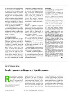
Fig. 8.1. Neural network-based hyperspectral data classification

Neural networks have been widely used in previous work to analyze hyperspectral images [3]. In particular, neural architectures have demonstrated great potential to model mixed pixels, which result from limited spatial resolution in certain application domains and also from the mixed nature of the interaction between photons and particles of observed land-cover surfaces. Since this process is inherently nonlinear, neural networks are an appropriate tool for mixed pixel classification due to their capacity to approximate complex nonlinear functions [4]. The standard classification approach adopted for neural networks is illustrated in Fig. 8.1, in which the original input data is first reduced in its dimensionality to avoid the Hughes effect. Previous research has demonstrated that the highdimensional data space spanned by hyperspectral data sets is usually empty [5], indicating that the data structure involved exists primarily in a subspace. Commonly used techniques to reduce the dimensionality of the data have been the principal component transform (PCT) or the minimum noise fraction (MNF) [6]. The discrete wavelet transform (DWT) or independent component analysis (ICA) have also been proposed for this task [7]. However, these approaches rely on spectral properties of the data alone, thus neglecting the information related to the spatial arrangement of the pixels in the scene. Usually, we need to manage very highdimensional data volumes in which spatial correlation between spectral responses of neighboring pixels can be potentially high [8]. As a result, there is a need for feature extraction techniques able to integrate the spatial and spectral information available from the data simultaneously [7]. Once a set of relevant features have been extracted from the input data, artificial neural network-based classification usually follows a supervised strategy, in which a few randomly selected training samples are selected from available labeled data and used to train the neural classifier. The trained classifier is then tested using the remaining samples.

8 Parallel Classification of Hyperspectral Images Using Neural Networks

195

Although many neural network architectures have been explored in the literature, feedforward networks of various layers, such as the multi-layer perceptron (MLP), have been widely used in hyperspectral imaging applications [9]. The MLP is typically trained using the error back-propagation algorithm, a supervised technique of training with three phases. In the first one, an initial vector is presented to the network, which leads to the activation of the network as a whole. The second phase computes an error between the output vector and a vector of desired values for each output unit, and propagates it successively back through the network. The last phase computes the changes for the connection weights, which are randomly generated at the beginning of the process. It has been shown in the literature that MLP-based neural models, when trained accordingly, generally outperform other nonlinear models such as regression trees or fuzzy classifiers [9]. Despite the success of neural network models for classification of remotely sensed hyperspectral images, several challenges still remain open in order to incorporate such models to real applications. An important limitation of these models is the fact that their computational complexity can be quite high [10], in particular, when they are used to analyze large hyperspectral data sets (or data repositories) comprising hundreds of spectral channels per scene [4]. To address the computational needs introduced by neural network-based algorithms in hyperspectral imaging applications, several efforts have been recently directed towards the incorporation of parallel computing models in remote sensing, specially with the advent of relatively cheap Beoulf clusters [11], [12]. The goal is to create parallel computing systems from commodity components to satisfy specific requirements for the Earth and space sciences community [13]. Although most dedicated parallel machines employed by NASA and other institutions during the last decade have been chiefly homogeneous in nature [14], a current trend is to utilize heterogeneous and distributed parallel computing platforms [15]. In particular, computing on heterogeneous networks of computers (HNOCs) is an economical alternative which can benefit from local (user) computing resources while, at the same time, achieve high communication speed at lower prices. These properties have led HNOCs to become a standard tool for high-performance computing in many ongoing and planned remote sensing missions [16], [17], thus taking advantage of from the considerable amount of work done in dynamic, resource-aware static and dynamic task scheduling and load balancing in distributed platforms, including distributed systems and Grid computing environments. Despite the increasing importance of HNOCs in remote sensing data interpretation, there is a lack of consolidated neural network-based algorithms specifically developed for heterogeneous computing platforms. To address the need for cost-effective and innovative parallel neural network classification algorithms, this chapter develops a new morphological/neural parallel algorithm for classification of hyperspectral imagery. The algorithm is inspired by previous work on morphological neural networks, such as autoassociative morphological memories and morphological perceptrons [18], although it is based on different concepts.

196

J. Plaza et al.

Most importantly, the algorithm can be tuned for very efficient execution on both HNOCs and massively parallel, Beowulf-type commodity clusters. The remainder of the chapter is structured as follows. Section 8.2 describes the proposed heterogeneous parallel algorithm, which consists of two main processing steps: 1) parallel morphological feature extraction taking into account the spatial and spectral information, and 2) robust classification using a parallel multi-layer neural network with back-propagation learning. Section 8.3 describes the algorithm’s accuracy and parallel performance. Classification accuracy is discussed in the context of a real applications, including land-cover classification of agricultural fields in the valley of Salinas, California and urban classification using hyperspectral data collected over the city of Pavia, Italy. Parallel performance in the context of the above-mentioned application is also provided by comparing the efficiency achieved by an heterogeneous parallel version of the proposed algorithm, executed on a fully heterogeneous network, with the efficiency achieved by its equivalent homogeneous version, executed on a fully homogeneous network with the same aggregate performance as the heterogeneous one. For comparative purposes, performance data on Thunderhead, a massively parallel Beowulf cluster at NASA’s Goddard Space Flight Center, are also given. Finally, Section 8.4 concludes with some remarks and hints at plausible future research.

8.2 Parallel Morphological/Neural Classification Algorithm In this section we present a new parallel approach for neural network-based classification of hyperspectral data, which has been specifically tuned for efficient execution in heterogeneous parallel platforms. The section is structured as follows. First, we formulate a general optimization problem in the context of HNOCs. Then, we separately describe the two main steps of the proposed parallel neural algorithm. The first stage (morphological feature extraction) relies on a feature selection stage performed by using extended morphological operations specifically tuned to deal with hyperspectral images. The second stage (neural network classification) is a supervised technique in which the extracted features are fed to a MLP-based neural architecture and used to classify the data according to a gradient descent algorithm. 8.2.1

Optimization Problem

Heterogeneous networks are composed of different-speed processors that communicate through links at different capacities [15]. This type of platform can be simply modeled as a complete graph G = (P, E) where each node models a computing resource pi weighted by its relative cycle-time wi . Each edge in the graph models a communication link weighted by its relative capacity, where cij denotes the maximum capacity of the slowest link in the path of physical communication links from pi to pj . We also assume that the system has symmetric costs, i.e., cij = cji . Under the above assumptions, processor pi will accomplish a share


197

P of αi × W of the total workload W , with αi ≥ 0 for 1 ≤ i ≤ P and i=1 αi = 1. With the above assumptions in mind, an abstract view of our problem can be simply stated in the form of a client-server architecture, in which the server is responsible for the efficient distribution of work among the P nodes, and the clients operate with the spatial and spectral information contained in a local partition. The partitions are then updated locally and the resulting calculations may also be exchanged between the clients, or between the server and the clients. Below, we describe the two main steps of our parallel algorithm. 8.2.2

Parallel Morphological Feature Extraction

This section develops a parallel morphological feature extraction algorithm for hyperspectral image analysis. First, we describe the morphological algorithm and its principles, then we study several possibilities for its parallel implementation for HNOCs. Morphological feature extraction algorithm The feature extraction algorithm presented in this section is based on concepts from mathematical morphology theory [19], which provides a remarkable framework to achieve the desired integration of the complementary nature of spatial and spectral information in simultaneous fashion, thus alleviating the problems related to each of them taken separately. In order to extend classical morphological operations from gray-scale image analysis to hyperspectral image scenarios, the main goal is to impose an ordering relation (in terms of spectral purity) in the set of pixel vectors lying within a spatial search window (called structuring element) designed by B [7]. This is done by defining a cumulative distance between a pixel vector f(x, y) and all the pixel vectors in the neighborhood given by spatial B (B -neighborhood) as follows: DB [f(x, y)] = i j SAD[f(x, y), f(i, j)], where (x, y) refers to the spatial coordinates in the B -neighborhood and SAD is the spectral angle distance, given by the following expression: f(x, y) · f(i, j) SAD(f(x, y), f(i, j)) = arccos . (8.1) f(x, y) · f(i, j) From the above definitions, two standard morphological operations called extended erosion and dilation can be respectively defined as follows: (f ⊗ B)(x, y) = argmin(s,t)∈Z 2 (B)

s

(f ⊕ B)(x, y) = argmax(s,t)∈Z 2 (B)

SAD(f (x, y), f (x + s, y + t)),

s

(8.2)

t

SAD(f(x, y), f(x − s, y − t)).

(8.3)

t

Using the above operations, the opening filter is defined as (f◦B)(x, y) = [(f⊗ B) ⊕ B](x, y) (erosion followed by dilation), while the closing filter is defined as

198

J. Plaza et al.

(f • B)(x, y) = [(f ⊕ B) ⊗ B](x, y) (dilation followed by erosion). The composition of opening and closing operations is called a spatial/spectral profile, which is defined as a vector which stores the relative spectral variation for every step of an increasing series. Let us denote by {(f ◦ B)λ (x, y)}, withλ = {0, 1, ..., k}, the opening series at f(x, y), meaning that several consecutive opening filters are applied using the same window B. Similarly, let us denote by {(f•B)λ (x, y)}, λ = {0, 1, ..., k}, the closing series at f(x, y). Then, the spatial/spectral profile at f(x, y) is given by the following vector: p(x, y) = {SAM((f ◦ B)λ (x, y), (f ◦ B)λ−1 (x, y))} ∪ · · · · · · ∪ {SAM((f • B)λ (x, y), (f • B)λ−1 (x, y))}. (8.4) Here, the step of the opening/closing series iteration at which the spatial/spectral profile provides a maximum value gives an intuitive idea of both the spectral and spatial distribution in the B -neighborhood [7]. As a result, the morphological profile can be used as a feature vector on which the classification is performed using a spatial/spectral criterion. Parallel implementations Two types of data partitioning can be exploited in the parallelization of spatial/spectral algorithms such as the one addressed above [14]: 1. Spectral-domain partitioning. Subdivides the volume into small cells or sub-volumes made up of contiguous spectral bands, and assigns one or more sub-volumes to each processor. With this model, each pixel vector is split amongst several processors, which breaks the spectral identity of the data because the calculations for each pixel vector (e.g., for the SAD calculation) need to originate from several different processing units. 2. Spatial-domain partitioning. Provides data chunks in which the same pixel vector is never partitioned among several processors. As a result, each pixel vector is always entirely stored in the same processing unit, thus entirely preserving the full spectral signature associated to the pixel at the same processor. In this chapter, we adopt a spatial-domain partitioning approach due to several reasons. First and foremost, the application of spatial-domain partitioning is a natural approach for morphological image processing, as many operations require the same function to be applied to a small set of elements around each data element present in the image data structure, as indicated in the previous subsection. A second reason has to do with the cost of inter-processor communication. For instance, in spectral-domain partitioning, the structuring element-based calculations made for each hyperspectral pixel would need to originate from several processing elements, thus requiring intensive inter-processor communication. However, if redundant information such as an overlap border is added to each of


199

the adjacent partitions to avoid accesses outside the image domain, then boundary data to be communicated between neighboring processors can be greatly minimized. Such an overlapping scatter would obviously introduce redundant computations, since the intersection between partitions would be non-empty. Our implementation makes use of a constant structuring element B (with size of 3 × 3 pixels) which is repeatedly iterated to increase the spatial context, and the total amount of redundant information is minimized. To do so, we have implemented three different approximations in order to handle with these so-called border pixels: • MP-1 implements a non-overlapping scatter operation followed by overlap communication for every hyperspectral pixel vector, thus communicating small sets of pixels very often. • MP-2 implements a standard non-overlapping scatter operation followed by a special overlap communication which sends all border pixels beforehand , but only once. • MP-3 performs a special ’overlapping scatter’ operation that also sends out the overlap border data as part of the scatter operation itself (i.e., redundant computations replace communications). Here, we make use of MPI derived datatypes to directly scatter hyperspectral data structures, which may be stored non-contiguously in memory, in a single communication step. A pseudo-code of the proposed parallel morphological feature extraction algorithm is given below. The inputs to the algorithm are an N -dimensional cube f, and a structuring element B. The output is a set of morphological profiles for each pixel. 1. Obtain information about the heterogeneous system, including the number of processors, P , each processors identification number, {pi }P i=1 , and processor cycle-times, {wi }P i=1 . 2. Using B and the information obtained in step 1, determine the total volume of information, R, that needs to be replicated from the original data volume, V , according to the data communication strategies outlined above, and let the total workload W to be handled by the algorithm be given by W = V +R. Then, partition the data using one of the three considered partitioning strategies for morphological processing: MP-1, MP-2 or MP-3. i)

for all i ∈ {1, ..., P }. 3. Set αi = P(P/w (1/wi ) i=1 P 4. For m = i=1 αi to (V + R), find k ∈ {1, .., P } so that wk · (αk + 1) = min{wi · (αi + 1)}P i=1 and set αk = αk + 1. 5. Use the resulting {αi }P i=1 to obtain a set of P spatial-domain heterogeneous partitions of W in accordance with the selected strategy: MP-1, MP-2 or MP-3, and send each partition to processor pi , along with B. 6. Calculate the morphological profiles p(x, y) for the pixels in the local data partitions (in parallel) at each heterogeneous processor. 7. Collect all the individual results and merge them together to produce the final output at the master processor.

200

J. Plaza et al.

It should be noted that a homogeneous version of the algorithm above can be simply obtained by replacing step 4 with αi = P/wi for all i ∈ {1, ..., P }, where wi is the communication speed between processor pairs in the network, assumed to be homogeneous. 8.2.3

Parallel Neural Classification Algorithm

The second step of the proposed parallel algorithm consists of a supervised parallel classifier based on a MLP neural network with back-propagation learning. The neural network is trained with selected features from the previous morphological feature extraction. This approach has been shown in previous work to be very robust for classification of hyperspectral imagery [20]. However, the considered neural architecture and back-propagation-type learning algorithm introduce additional considerations for parallel implementation on HNOCs. This section first describes the neural network architecture and learning procedure, and then describes several strategies for its parallelization, resulting in two main approaches for efficient implementation in HNOCs, namely, Exemplar partitioning and Hybrid partitioning. Network architecture and learning The architecture adopted for the proposed MLP-based neural network classifier is shown in Fig. 8.2. The number of input neurons equals the number of spectral bands acquired by the sensor. In case either PCT-based pre-processing or morphological feature extraction are applied as a pre-processing steps, then the number of neurons at the input layer equals the dimensionality of feature vectors used for classification. The second layer is the hidden layer, where the number of nodes, M , is usually estimated empirically. Finally, the number of neurons at the output layer, C, equals the number of distinct classes to be identified in the input data. With the above architecture, the activation function for hidden and output nodes can be selected by the user. In this chapter, we have used sigmoid activation for all experiments. With the above architectural design in mind, the standard back-propagation learning algorithm can be outlined by the following steps: 1. Forward phase. Let the individual components of an input pattern be denoted by fj (x, y), with j = 1, 2, ..., N . The output of the neurons at the hidden layer N are obtained as: Hi = ϕ( j=1 ωij · fj (x, y)) with i = 1, 2, ..., M , where ϕ(·) is the activation function and ωij is the weight associated to the connection between the i-th input node and the Mj -th hidden node. The outputs of the MLP are obtained using Ok = ϕ( i=1 ωki · Hi ), with k = 1, 2, ..., C. Here, ωki is the weight associated to the connection between the i-th hidden node and the k -th output node. 2. Error back-propagation. In this stage, the differences between the desired and obtained network outputs are calculated and back-propagated. The delta terms for every node in the output layer are calculated using δko = (Ok − dk ) ·


201

Fig. 8.2. MLP neural network topology

ϕ (·), with i = 1, 2, ..., C. Here, ϕ (·) is the first derivative of the activation function. Similarly, delta terms for the hidden nodes are obtained using δih = C o k=1 (ωki · δi ) · ϕ(·)), with i = 1, 2, ..., M . 3. Weight update. After the back-propagation step, all the weights of the network need to be updated according to the delta terms and to η, a learning rate parameter. This is done using ωij = ωij + η · δih · fj (x, y) and ωki = ωki + η · δko · Hi . Once this stage is accomplished, another training pattern is presented to the network and the procedure is repeated for all incoming training patterns. Once the back-propagation learning algorithm is finalized, a classification stage follows, in which each test input pixel vector is classified using the weights obtained by the network during the training stage [20]. Diffferent strategies for parallel classification using the proposed MLP architecture are given in the following subsection. Parallel MLP classification Several partitioning schemes can be analyzed when mapping a MLP neural network on a cluster architecture [21]. The choice is application-dependent, and a key issue is the number of training patterns to be used during the learning stage. In this chapter, we present two different schemes for the multi-layer perceptron classifier partitioning: 1. Exemplar partitioning. This approach, also called training example parallelism, explores data level parallelism and can be easily obtained by simply partitioning the training pattern data set (see Fig. 8.3). Each process determines the weight changes for a disjoint subset of the training population and then changes are combined and applied to the neural network at the end of each epoch. As will be shown by experiments, this scheme requires

202

J. Plaza et al.

Fig. 8.3. Exemplar partitioning scheme over MLP topology. Training data is divided into different subsets which are used to train three different subnetworks, i.e., white, grey and black.

a large number of training patterns to produce significant speedups, which is the most common situation in most remote sensing applications due to the limited availability of training samples and the great difficulty to generate accurately labeled ground-truth samples prior to analyzing the collected data. 2. Hybrid partitioning. This approach is based on a combination of neuronal level as well as synaptic level parallelism [22] which allows us to reduce the processor intercommunications at each iteration (see Fig. 8.4). This approach results from a combination of neuronal level parallelism and synaptic level parallelism. In the former (also called vertical partitioning) all the incoming weights to the neurons local to the processor are computed by a single processor. In the latter, each workstation will compute only the outgoing weight connections of the nodes (neurons) local to the processor. The hybrid scheme combines those approaches, i.e., the hidden layer is partitioned using neuronal parallelism while weight connections adopt synaptic scheme. As a result, all inter-processor communications will be reduced to a cumulative sum at each epoch, thus significantly reducing processing time on parallel platforms. Implementation of parallel Exemplar partitioning As mentioned above, the exemplar parallelism strategy is relatively easy to implement. It only requires the addition of an initialization algorithm and a synchronization step on each iteration. The initialization procedure distribute the


203

training patterns among the different processors according to their relative speed and memory characteristics. As shown in Fig. 8.3, each processor will implement a complete neural network topology which will compute only the previously related pattern subset. On each iteration, a synchronization step is required in order to integrate the weights matrices actualization obtained at each MLP architecture considering its respective training pattern subset. It can be easily achieved by having all the processors communicate their partial weights change matrices to the master node which computes the total sum of all partial matrices and applies the changes to the network. It then broadcasts the new weights matrix to the slave nodes. In our approximation, we improve the communication task by taking advantage of MPI predefined communication directives, which allow us to perform an all to all actualization and communication in a single MPI directive. A pseudo-code of the Exemplar partitioning algorithm can be summarized as follows. The inputs to the algorithm are an N -dimensional cube f, and a set of training patterns fj (x, y). The output is a classification label for each image pixel. 1. Use steps 1-4 of the parallel morphological feature extraction algorithm to obtain a set of values (αi )P i=1 which will determine the share of the workload to be accomplished by each heterogeneous processor. 2. Use the resulting (αi )P i=1 to obtain a set of P heterogeneous partitions of the training patterns and map the resulting partitions fP j (x, y) among the P heterogeneous processors (which also store the full multi-layer perceptron architecture). 3. Parallel training. For each training pattern contained on each partition, the following three steps are executed in parallel for each processor: a) Parallel forward phase. In this phase, the activation value of the hidden neurons local to the processors are calculated. For each input pattern, the activation value for the hidden neurons is calculated using HiP = N ϕ( j=1 ωij · fP j (x, y)). Here the activation values of output neurons are M P · HiP ), with k = 1, 2, ..., C. calculated according to OkP = ϕ( i=1 ωki b) Parallel error back-propagation. In this phase, each processor calculates the error terms for the local training patters. To do so, delta terms for the output neurons are first calculated using (δko )P = (Ok − dk )P · ϕ (·), with i = 1, 2, ..., Then, error terms for the hidden layer are computed C. P P · (δko )P ) · ϕ (·), with i = 1, 2, ..., N . using (δih )P = k=1 (ωki c) Parallel weight update. In this phase, the weight connections between the input and hidden layers are updated by ωij = ωij + η P · (δih )P · fP j (x, y). Similarly, the weight connections between the hidden and output layers P P are updated using ωki = ωki + η P · (δko )P · HiP . d) Broadcast and intialization of weight matrices. In this phase, each node sends its partial weight matrices to its neighbor node, which sums it to its partial matrix and proceed to send it again to the neighbor. When all nodes have added their local matrices, then the resulting total weight matrices are broadcast to be used by all processors in the next iteration.

204

J. Plaza et al.

4. Classification. For each pixel vector in the input data cube f, calculate (in j parallel) P j=1 Ok , with k = 1, 2, ..., C. A classification label for each pixel can be obtained using the winner-take-all criterion commonly used in neural network sum with maximum value, P P applications by finding the cumulative say j=1 Okj ∗ , with k ∗ = arg{max1≤k≤C j=1 Okj }. Implementation of parallel Hybrid partitioning In the hybrid classifier, the hidden layer is partitioned so that each heterogeneous processor receives a number of hidden neurons which depends on its relative speed. Figure 8.4 shows how each processor stores the weight connections between the neurons local to the processor. Since the fully connected MLP network is partitioned into P partitions and then mapped onto P heterogeneous processors using the above framework, each processor is required to communicate with every other processor to simulate the complete network. For this purpose, each of the processors in the network executes the three phases of the back-propagation learning algorithm described above. A pseudo-code of the Hybrid partitioning algorithm can be summarized as follows. The inputs to the algorithm are an N -dimensional data cube f, and a set of training patterns fj (x, y). The output is a classification label for each image pixel. 1. Use steps 1-4 of the parallel morphological feature extraction algorithm to obtain a set of values (αi )P i=1 which will determine the share of the workload to be accomplished by each heterogeneous processor. 2. Use the resulting (αi )P i=1 to obtain a set of P heterogeneous partitions of the hidden layer and map the resulting partitions among the P heterogeneous processors (which also store the full input and output layers along with all connections involving local neurons). 3. Parallel training. For each considered training pattern, the following three parallel steps are executed: a) Parallel forward phase. In this phase, the activation value of the hidden neurons local to the processors are calculated. For each input pattern, the activation value for the hidden neurons is calculated using HiP = N ϕ( j=1 ωij ·fj (x, y)). Here, the activation values and weight connections of neurons present in other processors are required to calculate the actiM/P P · HiP ), vation values of output neurons according to OkP = ϕ( i=1 ωki with k = 1, 2, ..., C. In our implementation, broadcasting the weights and activation values is circumvented by calculating the partial sum of the activation values of the output neurons. b) Parallel error back-propagation. In this phase, each processor calculates the error terms for the local hidden neurons. To do so, delta terms for the output neurons are first calculated using the formula (δko )P = (Ok − dk )P · ϕ (·), with i = 1, 2, ..., C. Then, error terms for the hidden layer P o P are computed using (δih )P = P k=1 (ωki ·(δk ) )·ϕ (·), with i = 1, 2, ..., N .


205

Fig. 8.4. Hybrid partitioning scheme over MLP topology. The input and output layers are common to all processors. The hidden nodes are distributed among different processors (lines, dotted-lines and dashed-lines denote weight connections corresponding to three different processors).

c) Parallel weight update. In this phase, the weight connections between the input and hidden layers are updated by ωij = ωij + η P · (δih )P · fj (x, y). Similarly, the weight connections between the hidden and output layers P P = ωki + η P · (δko )P · HiP . are updated using the expression: ωki 4. Classification. For each pixel vector in the input data cube f, calculate (in j parallel) P j=1 Ok , with k = 1, 2, ..., C. A classification label for each pixel can be obtained using the winner-take-all criterion commonly usedin neural P networks by finding the cumulative sum with maximum value, say j=1 Okj ∗ , P with k ∗ = arg{max1≤k≤C j=1 Okj }.

8.3 Experimental Results This section provides an assessment of the effectiveness of the parallel algorithms described in section 2. The section is organized as follows. First, we describe the parallel computing platforms used in this chapter for evaluation purposes. Then, we provide performance data for the proposed parallel algorithms in the context of two real hyperspectral imaging applications. 8.3.1

Parallel Computing Platforms

Before describing the parallel systems used for evaluation in this chapter, we briefly outline a recent study [23] on performance analysis for heterogeneous algorithms that we have adopted in this work for evaluation purposes. Specifically, we assess the parallel performance of the proposed heterogeneous algorithms

206

J. Plaza et al.

Table 8.1. Specifications of processors in a heterogeneous network of computers at University of Maryland Processor Architecture Cycle-time Main memory identification description (secs/megaflop) (MB) p1 Free BSD – i386 Intel Pentium 4 0.0058 2048 Linux – Intel Xeon 0.0102 1024 p2 , p5 , p8 Linux – AMD Athlon 0.0026 7748 p3 Linux – Intel Xeon 0.0072 1024 p4 , p6 , p7 , p9 SunOS – SUNW UltraSparc-5 0.0451 512 p10 Linux – AMD Athlon 0.0131 2048 p11 − p16

Cache (KB) 1024 512 512 1024 2048 1024

using the basic postulate that these algorithms cannot be executed on a heterogeneous network faster than its homogeneous prototypes on the equivalent homogeneous network. Let us assume that a heterogeneous network consists of {pi }P i heterogeneous workstations with different cycle-times wi , which span m communication seg(j) ments {sj }m denotes the communication speed of segment sj . Simj=1 , where c (j)

ilarly, let p(j) be the number of processors that belong to sj , and let wt be the speed of the t -th processor connected to sj , where t = 1, ..., p(j) . Finally, let c(j,k) be the speed of the communication link between segments sj and sk , with j, k = 1, ..., m. According to [23], the above network can be considered equivalent to a homogeneous one made up of {qi }P i=1 processors with constant cycle-time and interconnected through a homogeneous communication network with speed c if the following expressions are satisfied: m c=

j=1

(j)

c(j) · [ p

(p(j) −1) ] 2

P (P −1) 2

m m +

j=1

m p(j) j=1

t=1

(j) · k=j+1 p P (P −1) 2

p(k) · c(j,k)

,

(8.5)

(j)

wt

, (8.6) P where equation (8.5) states that the average speed of point-to-point communications between processors {pi }P i=1 in the heterogeneous network should be equal to the speed of point-to-point communications between processors {qi }P i=1 in the homogeneous network, with both networks having the same number of processors. On the other hand, equation (8.6) states that the aggregate performance of processors {pi }P i=1 should be equal to the aggregate performance of processors . {qi }P i=1 We have configured two networks of workstations at University of Maryland to serve as sample networks for testing the performance of the proposed heterogeneous hyperspectral imaging algorithm. The networks are considered approximately equivalent under the above framework. In addition, we have also used a massively parallel Beowulf cluster at NASA’s Goddard Space Flight Center in Maryland to test the scalability of the proposed parallel algorithms in a w=


207

Table 8.2. Capacity of communication links (time in milliseconds to transfer a onemegabit message) between processors in the heterogeneous network at University of Maryland Processor p1 − p4 p5 − p8 p9 − p10 p11 − p16

p1 − p4 19.26 48.31 96.62 154.76

p5 − p8 48.31 17.65 48.31 106.45

p9 − p10 p11 − p16 96.62 154.76 48.31 106.45 16.38 58.14 58.14 14.05

large-scale parallel platform. A more detailed description of the parallel platforms used in this chapter follows: 1. Fully heterogeneous network. Consists of 16 different workstations, and four communication segments. Table 8.1 shows the properties of the 16 heterogeneous workstations, where processors {pi }4i=1 are attached to communication segment s1 , processors {pi }8i=5 communicate through s2 ,processors 16 {pi }10 i=9 are interconnected via s3 , and processors {pi }i=11 share the communication segment s4 . The communication links between the different segments {sj }4j=1 only support serial communication. For illustrative purposes, Table 8.2 also shows the capacity of all point-to-point communications in the heterogeneous network, expressed as the time in milliseconds to transfer a one-megabit message between each processor pair (pi , pj ) in the heterogeneous system. As noted, the communication network of the fully heterogeneous network consists of four relatively fast homogeneous communication segments, interconnected by three slower communication links with capacities c(1,2) = 29.05, c(2,3) = 48.31, c(3,4) = 58.14 in milliseconds, respectively. Although this is a simple architecture, it is also a quite typical and realistic one as well. 2. Fully homogeneous network. Consists of 16 identical Linux workstations {qi }16 i=1 with processor cycle-time of w = 0.0131 seconds per megaflop, interconnected via a homogeneous communication network where the capacity of links is c = 26.64 milliseconds. 3. Thunderhead Beowulf cluster. Consists of 268 dual 2.4 Ghz Intel 4 Xeon nodes, each with 1 GB of memory and 80 GB of hard disk (see http://thunderhead.gsfc.nasa.gov for additional details). The total disk space available in the system is 21.44 Tbyte, and the theoretical peak performance of the system is 2.5728 Tflops (1.2 Tflops on the Linpack benchmark). Along with the 568-processor computer core, Thunderhead has several nodes attached to the core with Myrinet 2000 connectivity (see Fig. 8.5). Our parallel algorithms were run from one of such nodes, called thunder1. The operating system is Linux Fedora Core, and MPICH was the message-passing library used (see http://www-unix.mcs.anl.gov/mpi/mpich).

208

J. Plaza et al.

Fig. 8.5. Thunderhead Beowulf cluster at NASA’s Goddard Space Flight Center

8.3.2

Performance Evaluation

Before empirically investigating the performance of the proposed parallel hyperspectral imaging algorithms in the five considered platforms, we describe two hyperspectral image scenes that will be used in experiments. 1. AVIRIS data. The first scene was collected by the 224-band AVIRIS sensor over Salinas Valley, California, and is characterized by high spatial resolution (3.7-meter pixels). The area covered comprises 512 lines by 217 samples. 20 bands were discarded previous to the analysis due to low signal-to-noise ratio in those bands. Fig. 6(a) shows the spectral band at 587 nm wavelength, and Fig. 8.6(b) shows the ground-truth map, in the form of a class assignment for each labeled pixel with 15 mutually exclusive ground-truth classes. As shown by Fig. 8.6(b), ground truth is available for nearly half of Salinas scene. The data set above represents a very challenging classification problem (due to the spectral similarity of most classes, discriminating among them is very difficult). This fact has made the scene a universal and widely used benchmark test site to validate classification accuracy of hyperspectral algorithms [7]. 2. DAIS 7915 data. The second hyperspectral data set used in experiments was collected by the DAIS 7915 airbone imaging spectrometer of the German Aerospace Agency (DLR). It was collected by a flight at 1500 meters altitude over the city of Pavia, Italy. The resulting scene has spatial resolution of 5 meters and size of 400 lines by 400 samples. Fig. 8.7(a) shows the image collected at 639 nm by DAIS 7915 imaging spectrometer, which reveals a dense residential area on one side of the river, as well as open areas and


209

Fig. 8.6. (a) AVIRIS data collected over Salinas Valley, California, at 587 nm. (b) Salinas land-cover ground classes for several areas of the scene. (c) Classification results using the proposed morphological/neural algorithm.

meadows on the other side. Ground-truth is available for several areas of the scene (see Fig. 8.7(b)). Following a previous research study on this scene [7], we take into account only 40 spectral bands of reflective energy, and thus skip thermal infrared and middle infrared bands above 1958 nm because of low signal to noise ratio in those bands. In order to test the accuracy of the proposed parallel morphological/neural classifier in the context of a land-cover classification of agricultural crop fields, a random sample of less than 2% of the pixels was chosen from the known ground truth of the two images described above. Morphological profiles were then constructed in parallel for the selected training samples using 10 iterations, which resulted in feature vectors with dimensionality of 20 (i.e., 10 structuring element iterations for the opening series and 10 iterations for the closing series). The resulting features were then used to train the parallel back-propagation neural network classifier with one hidden layer, where the number of hidden neurons was selected empirically as the square root of the product of the number of input features and information classes (several configurations of the hidden layer were tested and the one that gave the highest overall accuracies was reported). The trained classifier was then applied to the remaining 98% of labeled pixels in each considered scene, yielding the classification results shown qualitatively for visual evaluation in Fig. 8.6(c) and quantitatively in Table 8.3. For comparative purposes, the accuracies obtained using the full spectral information and PCT-reduced features as input to the neural classifier are also reported in Table 8.3. As shown by the table, morphological input features

210

J. Plaza et al.

Table 8.3. Individual and overall test classification accuracies (in percentage) achieved by the parallel neural classifier for the Salinas AVIRIS data using as input feature vectors: the full spectral information contained in the original hyperspectral image, PCT-based features, and morphological features AVIRIS Spectral PCT-based Morphological Salinas information features features Broccoli green weeds 1 93.28 90.03 95.69 Broccoli green weeds 2 92.33 89.27 95.02 Fallow 96.23 91.16 97.10 Fallow rough plow 96.51 91.90 96.78 Fallow smooth 93.72 93.21 97.63 Stubble 94.71 95.43 98.96 Celery 89.34 94.28 98.03 Grapes untrained 88.02 86.38 95.34 Soil vineyard develop 88.55 84.21 90.45 Corn senesced green weeds 82.46 75.33 87.54 Lettuce romaine 4 weeks 78.86 76.34 83.21 Lettuce romaine 5 weeks 82.14 77.80 91.35 Lettuce romaine 6 weeks 84.53 78.03 88.56 Lettuce romaine 7 weeks 84.85 81.54 86.57 Vineyard untrained 87.14 84.63 92.93 Overall accuracy 87.25 86.21 95.08

Fig. 8.7. (a) DAIS 1795 data collected at 1500m. over the city of Pavia, Italy, at 639 nm. (b) Pavia land-cover ground classes for several areas of the scene. (c) Classification results using the proposed morphological/neural algorithm.

substantially improve individual and overall classification accuracies with regards to PCT-based features and the full spectral information. This is not surprising since morphological operations use both spatial and spectral information as opposed to the other methods which rely on spectral information alone. In order to substantiate the performance of the parallel algorithms in a different (and perhaps more challenging) application domain, we repeated the experiments above using the DAIS 7915 hyperspectral scene collected over downtown Pavia, Italy. The classification results achieved by the proposed morphological/neural classification algorithm are visually displayed in Fig. 8.7(c), and


211

Table 8.4. Individual and overall test classification accuracies (in percentage) achieved by the morphological/neural classifier for the DAIS 7915 Pavia scene using as input feature vectors: the full spectral information contained in the original hyperspectral image, PCT-based features, and morphological features DAIS 7915 Spectral PCT-based Morphological Pavia information features features Water 87.30 86.17 100.00 Trees 94.64 97.62 98.72 Asphalt 97.79 84.48 98.88 Parking lot 83.82 81.93 71.77 Bitumen 86.11 75.48 98.68 Brick roofs 83.69 82.36 99.37 Meadow 88.88 89.86 92.61 Bare soil 79.85 84.68 95.11 Shadows 89.64 92.81 96.19 Overall accuracy 88.65 89.75 96.16

Table 8.5. Execution times and load balancing rates (in the parentheses) for the different alternatives tested in the implementation of the morphological and neural stages of the proposed parallel classifier Heterogeneous versions: Heterogeneous network: Homogeneous network: Homogeneous versions: Heterogeneous network: Homogeneous network:

Morphological stage MP-1 MP-2 MP-3 267 (1.13) 211 (1.02) 214 (1.03) 279 (1.15) 216 (1.03) 221 (1.04) MP-1 MP-2 MP-3 2871 (1.89) 2535 (1.75) 2261 (1.68) 265 (1.13) 209 (1.02) 212 (1.03)

Neural stage Exemplar Hybrid 156 (1.04) 125 (1.02) 178 (1.03) 141 (1.01) Exemplar Hybrid 1261 (1.69) 1123 (1.61) 152 (1.04) 121 (1.02)

quantitatively reported in the form of individual and overall test classification accuracies in Table 8.4. The results obtained in this example confirm our introspection that the use of spatial/spectral filtering prior to classification can substantially increase the results obtained using the full original spectral information or a reduced version of this spectral-based information using standard transformations such as the PCT. Although these results are promising from the viewpoint of classification accuracy, further analyses in terms of computational complexity are required to fully substantiate the suitability of the proposed parallel morphological/neural algorithm for being used in real application with time-critical constraints. To investigate the properties of the parallel morphological/neural classification algorithm developed in this chapter, the performance of its two main modules (morphological feature extraction and neural classification) was first tested by timing the program using the heterogeneous network and its equivalent homogeneous one. Since the proposed parallel morphological/neural classification algorithm is dominated by regular computations, and given the satisfactory classification results reported in two completely different application scenarios, only parallel performance results for the Pavia (DAIS 7195 data) scene will be provided in the following subsection for the sake of simplicity.

212

J. Plaza et al.

For illustrative purposes, Table 8.5 shows the execution times measured for morphological and neural heterogeneous algorithms and their respective homogeneous versions on the two HNOCs (homogeneous and heterogeneous) at University of Maryland. Three alternative implementations of the parallel morphological feature extraction algorithm (denoted as MP-1, MP-2 and MP-3) and two different implementations of the parallel neural classification algorithm (Exemplar and Hybrid) were tested. As expected, the execution times reported on Table 8.5 for morphological and neural heterogeneous algorithms and their respective homogeneous versions indicate that the heterogeneous implementations were able to adapt much better to the heterogeneous computing environment than the homogeneous ones, which were only able to perform satisfactorily on the homogeneous network. From Table 8.5, one can also see that the heterogeneous algorithms were always several times faster than their homogeneous counterparts in the heterogeneous network, while the homogeneous algorithms only slightly outperformed their heterogeneous counterparts in the homogeneous network. Interestingly, Table 8.5 also reveals that the performance of the heterogeneous algorithms on the heterogeneous network was almost the same as that evidenced by the equivalent homogeneous algorithms on the homogeneous network (i.e., the algorithms achieved essentially the same speed, but each on its network). This seems to indicate that the heterogeneous algorithms are very close to the optimal heterogeneous modification of the basic homogeneous ones. In order to measure load balance, Table 8.5 also shows (in the parentheses) the imbalance scores achieved by the different stages of the parallel algorithm on the two considered networks of workstations. The imbalance is simply defined as D = Rmax /Rmin , where Rmax and Rmin are the maxima and minima processor run times across all processors, respectively. Therefore, perfect balance is achieved when D = 1. As we can see from Table 8.5, the proposed heterogeneous implementations were all effective in terms of load balance in all cases except for MP-1 which communicates pixels too often. On the other hand, the homogeneous algorithms executed on the heterogeneous platforms achieved the worst load-balancing ratios as expected. For the sake of quantitative comparison, Table 8.6 reports the measured execution times achieved by all tested algorithms on Thunderhead, using different numbers of processors. It should be noted that the processing time measured for the sequential version of morphological feature extraction on one single Thunderhead node was 2057 seconds, while the processing time measured for the sequential version of the neural network classification stage was 1638 seconds. The parallel times reported on Table 8.6 reveal that the combination of MP-2 for spatial/spectral feature extraction, followed by the Hybrid neural classifier for robust classification is able to provide highly accurate hyperspectral classification results (in light of Tables 8.3 and 8.4), but also quickly enough for practical use. For instance, using 256 Thunderhead processors, the proposed classifier was able to provide a highly accurate classification for the Salinas AVIRIS scene in less than 20 seconds. In this regard, the measured processing times represent a significant improvement over commonly used processing strategies for this


213

Fig. 8.8. Scalability of parallel morphological feature extraction algorithms (MP-1, MP-2 and MP-3) and parallel neural classifiers (Exemplar and Hybrid) on Thunderhead. Table 8.6. Processing times in seconds and speedups (in the parentheses) achieved by multi-processor runs of the considered parallel algorithms on the Thunderhead Beowulf cluster at NASA’s Goddard Space Flight Center 4 16 MP-1 1177 (1.8) 339 (6.5) MP-2 797 (2.5) 203 (10.0) MP-3 826 (2.4) 215 (9.5) 2 4 Exmp. 1041 (1.9) 414 (4.8) Hyb. 973 (1.6) 458 (3.5)

36 146 (15.0) 79 (25.8) 88 (23.3) 8 248 (8.1) 222 (7.2)

64 100 81 (27.2) 53 (41.5) 39 (52.3) 23 (88.73) 45 (45.7) 27 (76.2) 16 32 174 (11.5) 142 (14.1) 114 (14.0) 55 (29.2)

144 42 (52.4) 17 (120.0) 20 (102.8) 64 99 (20.2) 27 (59.5)

196 37 (59.5) 13 (157.0) 16 (128.5) 128 120 (16.7) 15 (107.1)

256 36 (61.2) 10 (204.1) 12 (171.5) 256 120 (16.7) 7 (229.5)

kind of high-dimensional data sets, which can take up to more than one hour of computation for the considered problem size as evidenced by the sequential computation times reported above. Taking into account the results presented above, and with the ultimate goal of exploring issues of scalability (considered to be a highly desirable property in the design of heterogeneous parallel algorithms), we have also compared the speedups achieved by the heterogeneous algorithms on the Thunderhead Beowulf cluster. Fig. 8.8 plots the speedups achieved by multi-processor runs of the heterogeneous parallel implementations of the three developed versions of morphological feature extraction algorithms (MP-1, MP-2 and MP-3) over the corresponding single-processor runs of each considered algorithm on Thunderhead. Fig. 8.8 also shows similar results for the two presented parallel neural network classifiers (Exemplar and Hybrid). Although not displayed in Fig. 8.8, the scalability of homogeneous algorithms was essentially the same as that evidenced by their heterogeneous versions, with MP-2 and MP-3 showing scalability results close to linear and the expected slow down of MP-1 due to the great amount of small communications introduced, indicating that the ratio of communications to computations is progressively more significant as the number of processors is increased, and parallel performance is significantly degraded. The above results

214

J. Plaza et al.

clearly indicate that the proposed data-replication strategy is more appropriate than the tested data-communication strategy in the design of a parallel version of morphological feature extraction. As for parallel neural classifiers, the scalability of the Hybrid approach is very close to linear. As mentioned in previous sections, the Hybrid parallel method is based in the distribution of weight connections among different processors, which does not affect the basis of back-propagation learning algorithm. However, the speedup of Exemplar parallel method saturates for 64 processors and slightly declines afterwards. This is mainly due to the limited number of training patterns used during the training and the convergence problems resulting from the execution of several neural classifiers in parallel. It should be noticed that backpropagation algorithm is strongly dependent of the number of selected training patterns. Since the Exemplar method divides the total training pattern set into as many subsets as CPUs available, each local processing will likely have different local minima and convergence challenges, thus introducing load imbalance problems. According to our experimentation, the Exemplar approach is suitable for applications in which the number of available training patters is very high, which is often not the case in the context of remote sensing applications such as those discussed in this chapter.

8.4 Conclusions and Future Research In this chapter, we have presented several innovative parallel neural networkbased algorithms for hyperspectral image classification and implemented them on high performance computing platforms such as heterogeneous and homogeneous networks of workstations and commodity Beowulf clusters. As a case study of specific issues involved in the exploitation of heterogeneous algorithms for hyperspectral image information extraction, this work provided a detailed discussion on the effects that platform heterogeneity has on degrading parallel performance of a new morphological/neural classification algorithm, able to exploit the spatial and spectral information in simultaneous fashion. The proposed parallel classification approach was tested using hyperspectral data sets corresponding to real applications, such as a complex urban mapping scenario and an agricultural land-cover classification problem, both of which have been commonly used as benchmark test sites in the remote sensing community. The parallel performance evaluation strategy conducted in this work for assessing heterogeneous parallel algorithms was based on experimentally assessing each heterogeneous algorithm by comparing its efficiency on a fully heterogeneous network (made up of processing units with different speeds and highly heterogeneous communication links) with the efficiency achieved by its equivalent homogeneous version on an equally powerful homogeneous network. Scalability results on a massively parallel commodity cluster are also provided. Experimental results in this work anticipate that the combination of the (readily available) computational power offered by heterogeneous parallel platforms and the recent advances in the design of advanced parallel algorithms for


215

hyperspectral data classification algorithms (such as those presented in this work) may introduce substantial changes in the systems currently used for exploiting the sheer volume of hyperspectral data which is now being collected worldwide, on a daily basis. Although the experimental results presented in this chapter are encouraging, further work is still needed to arrive to optimal parallel design and implementations for the considered parallel algorithms. We also plan to implement the proposed parallel techniques on other massively parallel computing architectures, such as NASA’s Project Columbia and Grid computing environments. We are also developing implementations of the proposed algorithms on field programmable gate arrays (FPGAs) and commodity graphics processing units (GPUs), which represent a very appealing type of high performance hardware architecture for onboard hyperspectral image classification and compression.

Acknowledgement The authors would like to thank J. Dorband, J. C. Tilton and J. A. Gualtieri for many helpful discussions, and also for their support with experiments on NASA’s Thunderhead system. They also state their appreciation for Profs. M. Valero and F. Tirado.

References 1. Chang, C.I.: Hyperspectral imaging: techniques for spectral detection and classification. Kluwer, New York (2003) 2. Green, R.O., et al.: Imaging spectroscopy and the airborne visible/infrared imaging spectrometer (AVIRIS). Remote Sensing of Environment 65, 227–248 (1998) 3. Benediktsson, J.A., Swain, P.H., Ersoy, O.K.: Neural network approaches versus statistical methods in classification of multisource remote-sensing data. IEEE Trans. Geoscience and and Remote Sensing 28, 540–552 (1990) 4. Vilmann, T., Merenyi, E., Hammer, B.: Neural maps in remote sensing image analysis. Neural Networks 16, 389–403 (2003) 5. Landgrebe, D.A.: Signal theory methods in multispectral remote sensing. Wiley, Hoboken (2003) 6. Richards, J.A., Xia, J.: Remote sensing digital image analysis: an introduction, 4th edn. Springer, Berlin (2006) 7. Plaza, A., Martinez, P., Plaza, J., Perez, R.: Dimensionality reduction and classification of hyperspectral image data using sequences of extended morphological transformations. IEEE Trans. Geoscience and Remote Sensing 43, 466–479 (2005) 8. Plaza, A., Benediktsson, J.A., Boardman, J., Brazile, J., Bruzzone, L., CampsValls, G., Chanussot, J., Fauvel, M., Gamba, P., Gualtieri, J.A., Tilton, J.C., Trianni, G.: Advanced processing of hyperspectral images. In: Proceedings of the IEEE International Geoscience and Remote Sensing Symposium, pp. 1348–1351 (2006) 9. Baraldi, A., Binaghi, E., Blonda, P., Brivio, P.A., Rampini, A.: Comparison of the multilayer perceptron with neuro-fuzzy techniques in the estimation of cover class mixture in remotely sensed data. IEEE Trans. Geoscience and Remote Sensing 39, 994–1005 (2001)

216

J. Plaza et al.

10. Zhang, D., Pal, S.K.: Neural Networks and Systolic Array Design. World Scientific, Singapore (2001) 11. Sterling, T.: Beowulf cluster computing with Linux. MIT Press, Cambridge (2002) 12. Dorband, J., Palencia, J., Ranawake, U.: Commodity clusters at Goddard Space Flight Center. Journal of Space Communication 1, 227–248 (2003) 13. El-Ghazawi, T., Kaewpijit, S., Moigne, J.L.: Parallel and adaptive reduction of hyperspectral data to intrinsic dimensionality. In: Proceedings of the IEEE International Conference on Cluster Computing, pp. 102–109 (2001) 14. Plaza, A., Valencia, D., Plaza, J., Martinez, P.: Commodity cluster-based parallel processing of hyperspectral imagery. Journal of Parallel and Distributed Computing 66, 345–358 (2006) 15. Lastovetsky, A.: Parallel computing on heterogeneous networks. WileyInterscience, Hoboken (2003) 16. Aloisio, G., Cafaro, M.: A dynamic earth observation system. Parallel Computing 29, 1357–1362 (2003) 17. Wang, P., Liu, K.Y., Cwik, T., Green, R.O.: MODTRAN on supercomputers and parallel computers. Parallel Computing 28, 53–64 (2002) 18. Ritter, G.X., Sussner, P., Diaz, J.L.: Morphological associative memories. IEEE Transactions on Neural Networks 9, 281–293 (2004) 19. Soille, P.: Morphological image analysis: principles and applications. Springer, Berlin (2003) 20. Plaza, J., Plaza, A., Perez, R.M., Martinez, P.: Automated generation of semilabeled training samples for nonlinear neural network-based abundance estimation in hyperspectral data. In: Proceedings of the IEEE International Geoscience and Remote Sensing Symposium, pp. 345–350 (2005) 21. Plaza, J., Perez, R.M., Plaza, A., Martinez, P.: Parallel morphological/neural classification of remote sensing images using fully heterogeneous and homogeneous commodity clusters. In: Proceedings of the IEEE International Conference on Cluster Computing, pp. 328–337 (2006) 22. Suresh, S., Omkar, S.N., Mani, V.: Parallel implementation of back-propagation algorithm in networks of workstations. IEEE Transactions on Parallel and Distributed Systems 16, 24–34 (2005) 23. Lastovetsky, A., Reddy, R.: On performance analysis of heterogeneous parallel algorithms. Parallel Computing 30, 1195–1216 (2004)