A Bayesian method for model selection in environmental noise prediction
L. Martín-Fernández1*, D. P. Ruiz1, A. J. Torija2 and J. Míguez3
1Department 2Institute
of Applied Physics, University of Granada, Avda. Fuentenueva s/n, 18071 Granada, Spain
of Sound and Vibration Research, University of Southampton, Highfield,
3Department
Southampton SO17 1BJ, UK
of Signal Theory & Communications, Carlos III University of Madrid,
Avda. de la Universidad 30, Leganés, 28911 Madrid, Spain
*
Corresponding author:
[email protected]
1
ABSTRACT. Environmental noise prediction and modeling are key factors for addressing a
proper planning and management of urban sound environments. In this paper we propose a
maximum a posteriori (MAP) method to compare nonlinear state-space models that describe
the problem of predicting environmental sound levels. The numerical implementation of this method is based on particle filtering and we use a Markov chain Monte Carlo technique to
improve the resampling step. In order to demonstrate the validity of the proposed approach
for this particular problem, we have conducted a set of experiments where two prediction models are quantitatively compared using real noise measurement data collected in different urban areas.
Keywords: environmental noise level prediction, MAP model selection, Monte Carlo sampling,
nonlinear state-space model, particle filtering.
2
1
Introduction
Environmental noise is one of the most important environmental problems in urban
areas, since it has a great impact on the health and welfare of the exposed population (Laszlo et al., 2012). In urban agglomerations, road traffic is the main noise source and its effects on inhabitants are well known (Ouis, 2001; Dai et al., 2005). Several research works (e.g.,
Bjorkman, 1991; Lercher, 1996) have shown that noise affects daily activities and causes sleep disturbances. Therefore, in order to care for human health and provide dwellers with a
high quality of life, urban spaces should be planned with an appropriate sound environment, keeping noise levels under control.
The accurate characterization of the sound environment is essential for urban
planning. In urban areas there is a large variety of sound sources and conditions that, in turn, generate a wide variety of relevant acoustic situations. Thus, we can find locations with different composition of traffic, different urban settings, with presence of noise sources that
are difficult to characterize (e.g., business or leisure areas, works, ...), the existence of green
areas, etc., that create sound spaces with different sound pressure levels and with large differences in their temporal evolution and spectral composition.
Accordingly, the complexity of urban agglomerations makes the environmental noise
modeling and prediction a complex and nonlinear problem. Previous research has shown the influence of different variables on the characterization of the environmental noise level and in the description of the temporal evolution of the sound pressure level (Torija et al., 2007a;
Torija et al., 2007b; Torija et al., 2007c; Torija et al., 2010; Sachakamol et al., 2011). In the
literature, there are different methods and techniques that solve the problem of predicting environmental noise levels, from physical models to statistical models. For example, models
based on physical principles of sound generation and propagation, as Harmonoise/Imagine model (Watts, 2005), Calculation of Road Traffic Noise (CORTN) (Anon., 1975), Nord2000
(Kragh et al., 2002), etc., have an outstanding performance in estimating sound pressure levels. These models are mainly used for predicting long-term sound pressure levels from
road traffic but urban environments are characterized by the presence of other sound sources different than road traffic, such as leisure noise, commercial activities, etc., which have a great
influence in the generation of environmental noise in urban agglomerations. In Josse (1972),
Burgess (1977) and Bertoni et al. (1987) it is proposed to use statistical models. Although
these models can describe nonlinear correlations, they do not provide an accurate enough 3
approximation of the trend followed by the sound pressure level when this is affected by a
large number of physical parameters. Later on, in Cammarata et al. (1993), it is proposed to apply an artificial neural network (ANN) for noise prediction. The method involves the training of a backpropagation network (BPN) (McClelland and Rumelhart, 1988) using an
appropriate set of acoustic measurements and, in the subsequent phase, the network predicts the sound pressure level for various inputs. This method achieves good results because neural networks have a great capacity for approximating functions which are essentially nonlinear
(Lapedes and Farber, 1987; Suykens et al., 1996), as it is the environmental noise prediction problem. From this point of view, other authors have developed complex neural networks with the objective of providing a tool for the design, planning and evaluation of urban sound
environments and the ultimate goal of incorporating the needs of the population into the planning of urban agglomerations (Cammarata et al., 1995; Genaro et al., 2010; Torija et al., 2012).
Since several models may be available to describe the sound environment in a given
urban area, the question of how to choose the fittest model given a record of data arises
naturally. In this paper, we study dynamic models that can be put in a state-space form. In particular, we identify the sources of noise as the state variables of the model and allow them
to evolve randomly over time. The observations, or measurements, for the model are
indicators of the overall sound pressure level and 1/3-octave band sound levels (spectral
composition). The relationship between the observations (sound pressure levels) and the state variables (noise sources) is represented by nonlinearities (such as, e.g., different neural
network configurations (McClelland and Rumelhart, 1988)) and a random perturbation.
Given two state-space models, each one with a different nonlinear structure
describing the relationship between the indicators of sound pressure level and the noise sources, our goal is to quantify the fitness of each model to predict environmental noise levels
using a collection of real data sets and select the most suitable candidate. Following the
general approach in Djuric (1998), we propose to score the competing models by way of their
posterior probabilities conditional on the same data sets, i.e., we carry out maximum a
posteriori (MAP) model selection. Our approach involves the computation of the evidence (as
defined in MacKay (2003), Chapter 3) in favor of each one of the competing models. However,
since the models of interest are dynamic and nonlinear, these evidences cannot be found in closed form. To circumvent this difficulty, we introduce a numerical approximation method based on the use of particle filters (Gordon et al., 1993; Doucet et al., 2000; Doucet et al., 2001; 4
Djuric et al., 2003), similar to the model monitoring algorithm of Djuric (1999). The proposed
filtering algorithm includes Markov Chain Monte Carlo (MCMC) moves (Gilks and Berzuini, 2001) to mitigate the diversity loss that follows the resampling step in conventional particle filters. It should also be noted that the proposed method can be stated in terms of Bayes
factors (as defined in Bernardo and Smith (2009); see Chapter 6). In particular, when only
two models are compared, MAP selection as described in this paper corresponds to the Bayesian test in Proposition 6.1 of Bernardo and Smith (2009). Unlike Bayes factors, though,
the MAP scheme can also be applied in a straightforward manner when more than two models are competing.
This paper is organized as follows. In Section 2 we define the state-space models to be
compared. In Section 3 we elaborate on the MAP criterion for model selection. The particle
filtering algorithm applied for the numerical implementation is described in Section 4. In
Section 5 we compare the proposed MAP model selection scheme with other Bayesian
techniques for model selection. In Section 6 we test the proposed methodology by using a
series of measurements of sound pressure levels obtained experimentally in the city of Granada (Spain). The obtained results are shown and discussed here. Finally, the article ends
with a summary and some conclusions in Section 7.
2
2.1
Models
Sound pressure levels
Let us consider the problem of predicting the value of 23 descriptors of sound
pressure level in urban areas from the knowledge of a set of noise sources. To be specific, the indicators of interest are the A-weighted equivalent continuous sound pressure level, 𝐿𝐴𝑒𝑞
(57-85 dBA), the non-weighted equivalent continuous sound pressure level, 𝐿𝑒𝑞 (65-90 dB),
and the sound level in 1/3 octave bands from 40 Hz to 4 kHz, 𝐿𝑓 (10-80 dB), where 𝑓 = 40, 50, 63, 80, 100, 125, 160, 200, 250, 315, 400, 500, 630, 800, 1000, 1250, 1600, 2000, 2500,
3150 and 4000 Hz. These magnitudes have been obtained from field measurements with 𝑆
integration time (𝑆 = 2 minutes).
2.2
State variables
5
A precise characterization of the urban sound environment requires the consideration
of a wide range of different magnitudes related to the sound emission generated by the present sources of noise as well as the sound propagation in diverse geometrical
configurations. In this paper, we collectively refer to these magnitudes as state variables.
Specifically, we study 25 variables displayed in Table 1: 20 sound emission variables (entries 1-10, 16-25 in Table 1) and 5 sound propagation variables (entries 11-15 in Table 1). The
pavement type (entry 9 in Table 1) is also related to sound propagation because sound is
propagated differently in paved surfaces (sound reflection) and porous surfaces (sound
absorption) (Lui and Li, 2004). The selection and classification of the state variables is taken
from Torija et al. (2010). Note that most of state variables are static over time (entries 1-15 in
Table 1) except the type and magnitude of the traffic flows, the number of vehicles with sirens and impulsive sound events (Torija et al., 2011) (entries 16-25 in Table 1), which can change
significantly depending on both time and location. [Place Table 1 here]
2.3
Nonlinear prediction of sound pressure levels
The prediction of sound pressure levels from noise sources can be carried out by
different methods, e.g., physical models (Anon., 1975; Kragh et al., 2002; Watts, 2005) or
statistical models (Josse, 1972; Burgess, 1977; Bertoni et al., 1987). However, since the
relationship between the sound pressure level and the noise sources is highly nonlinear,
neural networks have been advocated as efficient tools in urban agglomerations in
Cammarata et al. (1995), Genaro et al. (2010) and Torija et al. (2012) because of their ability to approximate nonlinear functions (studied in, e.g., Lapedes and Farber (1987) and Suykens et al. (1996)).
In this paper, as prediction functions of the candidate models, we use two
backpropagation networks (McClelland and Rumelhart, 1988) with different configurations
(named Configuration 2 and Configuration 4 in Torija et al. (2012)). Nevertheless, note that
the proposed method could be applied to compare dynamical models based on other types of prediction functions. We have chosen these network configurations due to their similarity and
the difficulty of making an election a priori based on their goodness to fit data in different
locations.
In particular, the studied neural networks have a common structure, i.e., 2 layers with
25 inputs related to the state variables, 23 neurons in the hidden layers and 23 outputs 6
related to the sound pressure levels. Moreover, both nets use a hyperbolic tangent sigmoid transfer function (first layer) and a linear transfer function (second layer). However, they
were calibrated with different training functions. Both functions update the weight and bias
values according to the Levenberg-Marquardt optimization method (Marquardt, 1963; Hagan
and Menhaj, 1994) avoiding the nets overfit the experimental data, but the training of the first backpropagation network (network 1, in the sequel) uses a Bayesian regularization process
(MacKay, 1992; Foresee and Hagan, 1997) that is not applied when training the second network (network 2, in the sequel). The aim of this regularization algorithm is to improve the
generalization capability of the network and, then, obtain good results given new input data. In Torija et al. (2012), the network configuration 1 slightly outperformed the network configuration 2.
Both networks were trained using the same database, which covers the heterogeneity
of the city of Granada (Spain), a typical Southern Europe medium-sized city. The experimental
measurements, 274 records in total, were collected on working days, at different time periods,
in different urban settings and different traffic conditions by researchers of the laboratory of Physics and Environmental Acoustics (Department of Applied Physics, University of Granada). The main features of each location are outlined in Table 2. [Place Table 2 here]
The measurement of environmental noise was carried out in slots of 30 - 90 minutes,
with each experimental datum corresponding to a record of 2 minutes. According to that, in each collected time series, the first datum of, e.g, the “ascendant flow of light vehicles” (row 20
in Table 1) corresponds to the number of vehicles observed during the first two minutes, the second datum corresponds to the following two minutes, etc. For binary data, e.g., the
“impulsive sound event” of row 18 in Table 1, the first datum indicates whether at least one impulsive event was observed during minutes 1 and 2, the second datum corresponds to
minutes 3 and 4, and so on. Note that the short two-minute period was chosen to ease the observation of the short-term variability of the sound pressure level for each location. The measurements were obtained following international procedures of reference; all
microphones were mounted away from reflecting facades, at a height of 4 meters above local ground level (Directive 2002/49/EC, 2002).
2.4
State-space models
As explained in Section 2.2, several state variables of the problem (entries 16-25 in 7
Table 1) are time-varying. Therefore, any model aimed to predict the values of the sound
pressure levels from these variables (e.g., traffic flows) should take into account their dynamics in order to produce adequate results. A compact manner to jointly represent the
state variable dynamics and the nonlinear relationship between the variables and the indicators of sound pressure level is by way of a state-space model.
To be specific, in each one of our candidate state-space model, let 𝒙𝑡 = �𝑥1,𝑡 , . . . , 𝑥10,𝑡 �, 𝑡 = 0, 1, . . . , 𝑇,
(1)
be the vector of time-varying state variables (i.e., the type and magnitude of the traffic flows,
the number of vehicles with sirens and impulsive sound events), where 𝑥𝑖,𝑡 , 𝑖 = 1, . . . ,10,
corresponds to the (15 + 𝑖)-th entry of Table 1 (i.e., 𝑥1,𝑡 is the “type of traffic flow” and
𝑥10,𝑡 is the “descendant flow of motorcycles”) and 𝑇 is the number of time steps. We collect
the static variables (related to the period of day, the geometrical configuration, the number of
lanes, etc.) in a vector
𝜽 = (𝜃1 , 𝜃2 , . . . , 𝜃15 ),
where 𝜃1 , . . . , 𝜃15 correspond to entries 1-15 in Table 1.
(2)
The indicators of sound pressure level and its spectral composition are represented by
a 23 dimensional vector
𝒚𝑡 = (𝑦1,𝑡 , . . . , 𝑦23,𝑡 )
(3)
where 𝑦1,𝑡 represents the value of the 𝐿𝐴𝑒𝑞 indicator at time 𝑡, 𝑦2,𝑡 represents the 𝐿𝑒𝑞
indicator at time 𝑡 and 𝑦3,𝑡 , . . . , 𝑦23,𝑡 stand for the remaining indicators in 1/3 octave bands from 40 Hz to 4 kHz (see Section 2.1).
The dynamics of 𝒙𝑡 is independent of the static variables in 𝜽, but the sound
pressure levels in 𝒚𝑡 are modeled as a function of 𝒙𝑡 , 𝜽 and the prediction method (in this
case, a neural network), plus a random perturbation. In particular, we have two state-space
models of the form *
𝒙𝑡 ~ 𝑝(𝒙𝑡 |𝒙𝑡−1 ),
𝒚𝑡 ~ 𝑝(𝒚𝑡 |𝒙𝑡 , 𝜽, 𝑚),
(4)
(5)
where 𝑚 ∈ {1,2} is the model index, 𝑝(𝒙𝑡 |𝒙𝑡−1 ) describes the conditional distribution of the dynamic variables (in particular, we assume that every 𝑥𝑖,𝑡 is first order Markovian) and 𝑝(𝒚𝑡 |𝒙𝑡 , 𝜽, 𝑚) is the conditional density of the sound pressure levels given the state variables
* We use
𝑝 to denote probability functions, including densities and masses. The notation is argument-wise. For example, if 𝑥 and 𝑦 are continuous random variables, then 𝑝(𝑥) and 𝑝(𝑦) denote their probability density functions, possibly different. If 𝑥 is a discrete random variable, then 𝑝(𝑥) denotes its probability mass function. Conditional densities and masses are indicated in the obvious way, e.g., 𝑝(𝑥|𝑦). This notation is common in Bayesian analysis and the particle filtering literature.
8
and the neural network used for prediction (either network 1 or network 2, as indicated by 𝑚).
The conditional density of the sound pressure levels, often referred to as the
likelihood of the variables, is assumed to be Gaussian, namely
𝑝(𝒚𝑡 |𝒙𝑡 , 𝜽, 𝑚) = 𝒩 (𝒚𝑡 ; 𝑔𝑚 (𝒙𝑡 , 𝜽), 𝐃𝑚 )
(6)
where 𝒩(𝐳; 𝜇, 𝐂) denotes the (multivariate) Gaussian probability density function (pdf) of
z with mean vector 𝜇 and covariance matrix C, 𝑔𝑚 (𝒙𝑡 , 𝜽) represents the sound pressure levels predicted by the m-th neural network and 𝜎2 ⎡ 𝑚,1 ⎢0 𝐃𝑚 = ⎢ ⎢⋮ ⎣0
0 2 𝜎𝑚,2 ⋮ 0
… … ⋱ …
0 ⎤ 0 ⎥ ⎥ ⋮ ⎥ 2 𝜎𝑚,23 ⎦
2 is a diagonal covariance matrix with the marginal variances 𝜎𝑚,𝑗 , 𝑗 = 1, . . . ,23 fitted using
the experimental data and the predictions from the 𝑚-th neural network. The Gaussian
model is not a limitation of the method because it is straightforward to incorporate other distributions for modeling the likelihood of state variables (e.g., Gaussian mixture models (Don and Rees, 1985) or impulsive models (Garcia and Faus, 1991)).
The dynamic states 𝑥1,𝑡 , 𝑥2,𝑡 , 𝑥3,𝑡 and 𝑥4,𝑡 (type of traffic flow, number of vehicles
with sirens and impulsive sound events, respectively) are discrete first-order Markov chains with transition probabilities given by the matrices 0.23 ⎡0.05 ⎢ 0 𝑷1 = ⎢ 0.19 ⎢ ⎢0.03 ⎣0.19 0.42 𝑷3 = � 0.53
0.30 0.34 0.46 0,37 0.10 0 0.58� 0.47
0.05 0.17 0.17 0.08 0 0
0.11 0.16 0.37 0.31 0.07 0
0.12 0.28 0 0.05 0.55 0.25 0.77 and 𝑷4 = � 0.72
0.19 0 ⎤ ⎥ 0.99 0 ⎥ , 𝑷2 = � 1 0 ⎥ ⎥ 0.25 0.56⎦ 0.23 �, 0.28
0.01 �, 0
respectively *. For the continuous variables (traffic flows), 𝑥5,𝑡 , . . . , 𝑥10,𝑡 , we have chosen a simple random walk model of the form
𝑝(𝑥𝑖,𝑡 |𝑥𝑖,𝑡−1 ) = 𝒩(𝑥𝑖,𝑡 ; 𝑥𝑖,𝑡−1 , 𝛼𝑖2 ), 𝑖 = 5, . . . ,10,
(7)
where 𝛼𝑖2 is a variance fitted using the collected data. We assume that the state variables evolve independently over time, i.e., 𝑝(𝒙𝑡 |𝒙𝑡−1 ) = ∏10 𝑖=1 𝑝(𝑥𝑖,𝑡 |𝑥𝑖,𝑡−1 ).
*
𝑗
We assume that a discrete variable 𝑥𝑖,𝑡 can take the values described in the value-range column of Table 1. Let 𝑥𝑖 be the j-th
value in the range of variable 𝑥𝑖,𝑡. The entry in the k-th row, l-th column of 𝐏𝑖 , denoted 𝑥𝑖𝑙 |𝑥𝑖,𝑡−1 = 𝑥𝑖𝑘 ).
9
𝑘,𝑙 P𝑖 ,
is the probability mass 𝑝(𝑥𝑖,𝑡 =
These two models have been chosen because they show a good and similar behavior in
predicting sound pressure levels. For urban planning, the selection of the model with the best performance is important because, even if both models have similar accuracy, the difference
between predictions is not trivial in Environmental Acoustics and can imply a substantial increase in the annoyance of the inhabitants or in the quantity of affected population .
3
Criterion for model selection
The aim of this paper is to formally show how, following a general Bayesian approach
presented in Djuric (1998), it is possible to score, and then select, different state-space models
to predict the indicators of sound pressure level. We have explicitly defined two models in Section 2.4, but the criterion (and procedure) to be introduced can be easily extended to an
arbitrary number of candidate models and/or different models (i.e., with other model
variables, different types of nonlinear prediction functions, etc.). 𝑝(𝑚)
Let the index 𝑚 ∈ {1,2} refer to the state-space model. We assign a prior probability to
each
model
𝑚
and,
given
a
fixed
record
of
experimental
data
𝒚1:𝑇 = {𝒚1 , 𝒚2 , . . . , 𝒚 𝑇 }, we use 𝑝(𝑚|𝒚1:𝑇 , 𝜽) to denote the a posteriori probability mass of the model m given the data and the static variables in 𝜽. For the rest of this paper, we assume 𝜽
is known and leave the dependences on this fixed vector implicit. Therefore, we write 𝑝(𝑚|𝒚1:𝑇 ) for the posterior probability of the model 𝑚 and 𝑝(𝒚1:𝑇 |𝑚) = 𝑝(𝒚1:𝑇 |𝑚, 𝜽) for the associated likelihood.
A natural criterion to choose the model that best fits the data is to solve the problem 𝑚 � = arg max 𝑝(𝑚|𝒚1:𝑇 ),
(8)
𝑝(𝒚1:𝑇 |𝑚)𝑝(𝑚)
(9)
𝑚∈{1,2}
where 𝑚 � is the maximum a posteriori (MAP) model choice. For calculating 𝑝(𝑚|𝒚1:𝑇 ), we apply the Bayes’ theorem
𝑝(𝑚|𝒚1:𝑇 ) =
𝑝(𝒚1:𝑇 )
,
where 𝑝(𝒚1:𝑇 |𝑚) is the joint probability density of the observations 𝒚1:𝑇 , conditional on the model m, 𝑝(𝑚) is the prior probability of 𝑚 and 𝑝(𝒚1:𝑇 ) is the unconditional probability density of 𝒚1:𝑇 (which is constant with respect to 𝑚). After applying the chain rule to Eq. (9), we rewrite (8) as
𝑚 � = arg max ∏𝑇𝑘=1 𝑝(𝒚𝑘 |𝒚1:𝑘−1 , 𝑚)𝑝(𝑚), 𝑚∈{1,2}
10
(10)
where 𝑝(𝒚𝑘 |𝒚1:𝑘−1 , 𝑚) is the predictive probability density of the sound pressure level
indicators at time 𝑘 given the previous indicators and the model 𝑚, for 𝑘 = 1, . . , 𝑇. In order to ease the calculations, let us take the logarithm of the product in (10), to obtain 𝑚 � = arg max log�∏𝑇𝑘=1 𝑝(𝒚𝑘 |𝒚1:𝑘−1 , 𝑚 )𝑝(𝑚)� 𝑚∈{1,2}
= arg max �∑𝑇𝑘=1 log 𝑝(𝒚𝑘 |𝒚1:𝑘−1 , 𝑚) + log 𝑝(𝑚)�. 𝑚∈{1,2}
(11)
Notice that the optimization problems (8) and (11) are equivalent because log(𝑧) is a
monotonically increasing function. Finally, for notational convenience, we define the objective function
𝐽𝑚 (𝑇) = ∑𝑇𝑘=1 log 𝑝(𝒚𝑘 |𝒚1:𝑘−1 , 𝑚) + log 𝑝(𝑚)
(12)
𝑚 � = arg max 𝐽𝑚 (𝑇).
(13)
and reduce the model selection problem to choosing the index 𝑚 that yields the highest value of 𝐽𝑚 (𝑇), i.e.,
𝑚∈{1,2}
In many cases, it may be of interest to compare the candidate models in terms of their
ability to predict a scalar observation 𝑦𝑖,𝑡 , 𝑖 = 1, 2, …, instead of the joint vector 𝒚𝑡 (e.g., in order to determine the sensitivity of the model for a given sound pressure level). The
derivation of the MAP criterion is exactly the same as before. Namely, for the 𝑖-th observation, we select
where
𝑖 𝑚 � = arg max 𝐽𝑚 (𝑇),
(14)
𝑖 𝐽𝑚 (𝑇) = ∑𝑇𝑘=1 log 𝑝�𝑦𝑖,𝑘 �𝑦𝑖,1:𝑘−1 , 𝑚� + log 𝑝(𝑚).
(15)
𝑚∈{1,2}
The MAP selection method that we propose in this paper is summarized as: Initialization.
a. Obtain the prior probability mass function 𝑝(𝑚) for the indices 𝑚 ∈ {1,2}.
b. Let 𝐽𝑚 (0) = log 𝑝(𝑚), 𝑚 ∈ {1,2}.
Sequential update. For 𝑡 = 1, . . . , 𝑇,
a. Compute the predictive pdf 𝑝(𝒚𝑡 |𝒚1:𝑡−1 , 𝑚).
b. Update the objective function, 𝐽𝑚 (𝑡) = 𝐽𝑚 (𝑡 − 1) + log 𝑝(𝒚𝑡 |𝒚1:𝑡−1 , 𝑚).
Selection. Choose the model 𝑚 � = arg max 𝐽𝑚 (𝑇). 𝑚∈{1,2}
4
Numerical implementation 11
The model selection method introduced in Section 3 demands the evaluation of the
sequence of posterior pdf’s 𝑝(𝒚𝑡 |𝒚1:𝑡−1 , 𝑚), 𝑡 = 1, … , 𝑇, for each model. Unfortunately, due
to the nonlinearity 𝑔𝑚 (𝒙𝑡 , 𝜽) in Eq. (6), there is no closed-form expression for these
densities, which, therefore, have to be approximated numerically.
In this paper, we propose to carry out these approximations using particle filtering
(Gordon et al., 1993; Doucet et al., 2000). Specifically, we apply a variation of the standard
particle filter (Gordon et al., 1993; Doucet et al., 2001) that includes a Markov Chain Monte
Carlo (MCMC) move after the resampling step. The aim of this move is to enhance the
diversity of the particle set (Gilks and Berzuini, 2001). The specific MCMC technique we have
used in this paper is a Metropolis-Hastings algorithm, as described in Chib and Greenberg
(1995). The algorithm is described as follows:
(𝑖)
Initialization. Let 𝑀 be the number of particles. Draw 𝒙0 Recursive steps. For 𝑡 = 1, … , 𝑇:
from 𝑝(𝒙0 ), 𝑖 = 1, … , 𝑀.
(𝑖)
�(𝑖) a. Draw 𝒙 from 𝑝(𝒙𝑡 |𝒙𝑡−1 ), 𝑖 = 1, . . . , 𝑀. 𝑡
(𝑖) �(𝑖) b. Update the importance weights, 𝑤 �𝑡 = 𝑝(𝒚𝑡 |𝒙 𝑡 , 𝑚) , and normalize them, (𝑖)
𝑤𝑡
=
(𝑖)
𝑤 �𝑡
(𝑗)
∑𝑀 �𝑡 𝑗=1 𝑤
, 𝑖 = 1, . . . , 𝑀.
(𝑖) (𝑘) �(𝑘) c. Multinomial resampling: for 𝑖 = 1, . . . , 𝑀, let � 𝒙𝑡 = 𝒙 with probability 𝑤𝑡 , 𝑡
𝑘 ∈ {1, . . . , 𝑀}.
d. MCMC move: take one step of the Metropolis-Hastings method to generate 𝒙(𝑖) 𝑡 �(𝑖) from 𝒙 𝑡 , 𝑖 = 1, . . . , 𝑀.
Let 𝛿𝒙 denote the unit delta measure centered at 𝒙 and consider the two sets of
(𝑖) 𝑀 𝑀 �(𝑖) particles (samples in the state space) {𝒙 𝑡 }𝑖=1 and {𝒙𝑡 }𝑖=1 generated by the particle filter
at each time step 𝑡. We can construct two random measures, 1
1
∑𝑀 𝛿 (𝑖) (𝑑𝒙𝑡 ), 𝜋𝑀 (𝑑𝒙𝑡 |𝒚1:𝑡−1 , 𝑚) = 𝑀 ∑𝑀 (𝑖) (𝑑𝒙𝑡 ) and 𝜋𝑀 (𝑑𝒙𝑡 |𝒚1:𝑡 , 𝑚) = 𝑖=1 𝛿𝒙 � 𝑀 𝑖=1 𝒙 𝑡
𝑡
that enable the approximation of integrals with respect to 𝑝(𝒙𝑡 |𝒚1:𝑡−1 ) and 𝑝(𝒙𝑡 |𝒚1:𝑡 ), respectively. Indeed, for any integrable real function 𝑓 in the state-space, 𝑀
1 �(𝑖) � 𝑓(𝒙𝑡 )𝑝(𝒙𝑡 |𝒚1:𝑡−1 , 𝑚)𝑑𝒙𝑡 ≈ � 𝑓(𝒙𝑡 )𝜋𝑀 (𝑑𝒙𝑡 |𝒚1:𝑡−1 , 𝑚) = � 𝑓(𝒙 𝑡 ), 𝑀 𝑖=1
12
and
𝑀
1 � 𝑓(𝒙𝑡 )𝑝(𝒙𝑡 |𝒚1:𝑡 , 𝑚)𝑑𝒙𝑡 ≈ � 𝑓(𝒙𝑡 )𝜋𝑀 (𝑑𝒙𝑡 |𝒚1:𝑡 , 𝑚) = � 𝑓(𝒙(𝑖) 𝑡 ). 𝑀 𝑖=1
The asymptotic convergence (as 𝑀 → ∞) of such approximations can be guaranteed under
mild regularity assumptions (Crisan, 2001; Moral, 2004; Bain and Crisan, 2008). In particular,
we note that the predictive pdf’s 𝑝(𝒚𝑡 |𝒚1:𝑡−1 , 𝑚) can be written as integrals of the form 𝑝(𝒚𝑡 |𝒚1:𝑡−1 , 𝑚) = � 𝑝(𝒚𝑡 |𝒙𝑡 , 𝑚)𝑝(𝒙𝑡 |𝒚1:𝑡−1 , 𝑚)𝑑𝒙𝑡 , 𝑡 = 1, … , 𝑇,
and hence we compute their approximations as
𝑝𝑀 (𝒚𝑡 |𝒚1:𝑡−1 , 𝑚) ≈ 𝑝(𝒚𝑡 |𝒚1:𝑡−1 , 𝑚),
where
1
(𝑖)
�𝑡 ). 𝑝𝑀 (𝒚𝑡 |𝒚1:𝑡−1 , 𝑚) = ∫ 𝑝(𝒚𝑡 |𝒙𝑡 , 𝑚)𝜋𝑀 (𝑑𝒙𝑡 |𝒚1:𝑡−1 , 𝑚) = 𝑀 ∑𝑀 𝑖=1 𝑝(𝒚𝑡 |𝒙
(16)
𝐽𝑚 (𝑡) ≈ ∑𝑡𝑘=1 log(𝑝𝑀 (𝒚𝑘 |𝒚𝟏:𝒌−𝟏 , 𝑚)) + 𝑝(𝑚)
(17)
We use Eq. (16) for the computation of the objective functions 𝐽𝑚 (𝑡), 1 ≤ 𝑡 ≤ 𝑇, i.e., we let in all the experimental results to be shown in Section 6.
5 5.1
Comparison with other Bayesian methods for model
selection
Bayes factors
Given two competing models, 𝑚 ∈ {1,2}, and a sequence of observations 𝒚1:𝑇 , the
Bayes factor in favor of the model 𝑚 = 1 (and against 𝑚 = 2) is the ratio of model likelihoods (Bernardo and Smith, 2009; Definition 6.1) 𝑝(𝒚
|𝑚=1)
𝐵12 (𝒚1:𝑇 ) = 𝑝(𝒚1:𝑇 |𝑚=2), 1:𝑇
−1 ( 𝒚1:𝑇 ). Bayes factors are naturally compared to the ratio of prior model with 𝐵21 (𝒚1:𝑇 ) = 𝐵12
probabilities weighted by the loss or penalty associated to decision errors (see Proposition 6.1 in Bernardo and Smith (2009)). In particular, let 𝑙𝑖𝑗 be the penalty due to selecting
model 𝑚 = 𝑖 when the “true” model is 𝑚 = 𝑗. Then, model 𝑚 = 1 should be preferred over 𝑚 = 2 if, and only if,
𝑙
𝑝(𝑚=2)
𝐵12 (𝒚1:𝑇 ) < 𝑙12 × 𝑝(𝑚=1). 13
21
(18)
However, if 𝑙12 = 𝑙21 , then it is apparent that the criterion (18) reduces to the MAP criterion
in Eq. (14), since 𝐵12 (𝒚1:𝑇 ) < 𝑝(𝑚 = 2)⁄𝑝(𝑚 = 1) if, and only if, 𝑝(𝑚 = 1|𝒚1:𝑇 ) >
𝑝(𝑚 = 2|𝒚1:𝑇 ). When the penalties are not symmetric it is straightforward to redefine the
priors for the competing models as 𝑝�(𝑚 = 2) = 𝑙12 𝑝(𝑚 = 2) and then the prosed MAP
criterion (with priors 𝑝�(𝑚), 𝑚 ∈ {1,2}) is, again, equivalent to the criterion given by Eq.
(18).
While the Bayes factors may be a convenient tool for comparing two models, the MAP
criterion can be applied in a direct manner to problems involing many competing models.
5.2
Deviance information criterion
The deviance information criterion (DIC) (Spiegelhalter et al., 2002) has become a
popular tool for Bayesian model selection in the last decade. It relies on the computation of a deviance or discrepancy between the model and the available data. For the class of state-space model in Section 3, the deviance takes the form
𝐷(𝒙0:𝑇 , 𝑚 ) = −2 log 𝑝(𝒚1:𝑇 |𝒙0:𝑇 , 𝑚)
and the DIC criterion consists in choosing the value of 𝑚 for which the statistic 𝐷𝐼𝐶 (𝑚 ) = ∫ 𝐷(𝒙0:𝑇 , 𝑚 ) π(𝑑𝒙0:𝑇 |𝒚1:𝑇 ) + 𝑑𝑝
(19)
𝑑𝑝 = ∫ 𝐷(𝒙0:𝑇 , 𝑚 ) π(𝑑𝒙0:𝑇 |𝒚1:𝑇 ) − 𝐷(∫ 𝒙0:𝑇 π(𝑑𝒙0:𝑇 |𝒚1:𝑇 ) , 𝑚).
(20)
is minimum, where 𝑑𝑝 is a penalty term (that penalizes higher dimensional models) of the form
Obviously, the integrals in Eqs. (19) and (20) cannot be computed exactly, but we can
resort to the random measure
𝑀
1 𝜋𝑀 (𝑑𝒙0:𝑇 |𝒚1:𝑇 , 𝑚) = � 𝛿𝒙(𝑖) (𝑑𝒙0:𝑇 ) 𝑀 0:𝑇 𝑖=1
produced by the particle filter in order to approximate them.
Therforefore, a test based on the DIC criterion is, in principle, implementable.
However, it is straightforward to realize that the numerical implementation of the MAP model
selection technique is more efficient. Indeed, the implementation of the proposed MAP scheme only requires the approximation of the sequence of measures 𝜋(𝑑𝒙t|𝒚1:𝑡−1 , 𝑚) for model 𝑚 (namely, to be used in Eq. (16)), where 𝒙t is a 10 × 1 vector for every
𝑡 = 0,1, … , 𝑇. To implement the DIC scheme, on the contrary, we need to build an
approximation of 𝜋(𝑑𝒙0:𝑇 |𝒚1:𝑇 , 𝑚) for each 𝑚 , where the dimension of 𝒙0:𝑇 is 14
10(𝑇 + 1) × 1. It is well known that PF’s are efficient in the approximation of 𝜋(𝑑𝒙t|𝒚1:𝑡 , 𝑚)
but not for the approximation of the higher dimensional 𝜋(𝑑𝒙0:𝑇 |𝒚1:𝑇 , 𝑚); see, e.g. Doucet et al. (2000), Cappé et al. (2007) or Künsch (2013) for a dicussion. This can potentially impair
the computationn of the deviances for the competing models, specially (and paradoxically) as more data is accumulated.
6
Experimental results
The proposed comparison method is validated using the two ANN-based state-space
models defined in Section 2.4 and experimental data collected in the streets 2, 3 and 6 of Table
2. We have chosen these three streets because they present different traffic conditions and urban settings. The street number 2 is a large commercial area with high flow of heavy
vehicles, light vehicles, and motorcycles, the street number 3 has a great ascendant traffic slope and high flow of heavy vehicles, and the street number 2 is a narrow street with low traffic flow.
A priori, model 1 should be expected to obtain the best results because its prediction
function (network 1) has been calibrated using an additional Bayesian regularization process
which has been shown to improve the generalization capabilities in neural networks (MacKay,
1992; Foresee and Hagan, 1997). Moreover, in Torija et al. (2012), the configuration of
network 1 slightly outperformed the configuration of network 2, in terms of mean squared error (MSE) and linear regression.
In this paper, we assess the candidate models with the presented method in two ways.
First, we compare their ability to predict the 23 indicators of sound pressure level jointly and,
second, we evaluate their ability to predict 6 relevant scalar indicators individually. In each
case, we apply the proposed MAP selection method to the two competing models using 𝑀 = 500 samples in the particle filtering algorithm and data sequences of length 𝑇 = 25 time steps (2 minutes each). We consider the same prior probability, 𝑝(𝑚) = 0.5, for both models.
Moreover, we show the improvement of the best model (the model with the maximum
value of 𝐽(𝑇)) in all the experiments, i.e., we calculate the normalized difference between the
goodness indicators 𝐽(𝑇) of the candidate models in percentage, 15
𝐼𝑚𝑝𝑟𝑜𝑣𝑒𝑚𝑒𝑛𝑡 (%) = 100 ∗
6.1
|𝐽1 (𝑇) − 𝐽2 (𝑇)| ∙ |min(𝐽1 (𝑇), 𝐽2 (𝑇))|
Model comparison for the complete indicator set
In this first set of experiments, the observation vectors 𝒚1 , … , 𝒚 𝑇 are 23 dimensional,
as shown in Eq. (3), i.e., they contain all the indicators of sound pressure level described in Section 2.1. Using the particle approximation of Eq. (17), we have evaluated the objective function 𝐽𝑚 (𝑇), for the two competing models (𝑚 = 1 and 𝑚 = 2) using separately the time
series of data from streets 2, 3 and 6.
The results are displayed in Table 3. We observe that 𝐽1 (𝑇) > 𝐽2 (𝑇) for the three
data sets. Specifically, model 𝑚 = 1 attains an improvement of 22.5% for street number 2,
21.1% for street number 3 and 22.1% for street number 6. Therefore, model 𝑚 = 1 is the
MAP choice (𝑚 � = 1) for these three streets when the complete set of indicators (sound pressure level and its spectral composition) are considered. [Place Table 3 here]
Figure 1 shows the evolution of the objective functions 𝐽1 (𝑡) and 𝐽2 (𝑡) over time,
for 1 ≤ 𝑡 ≤ 𝑇 = 25 steps, for the three data sets corresponding to streets 2, 3 and 6, respectively. We observe that 𝐽1 (𝑡) > 𝐽2 (𝑡) for all, even small, 𝑡. Moreover, the gap 𝐽1 (𝑡) − 𝐽2 (𝑡) grows consistently over time, indicating that model 𝑚 = 1 is a better fit than
model 𝑚 = 2 for these data sets. [Place Figure 1 here]
This results confirm that the model which uses the neural network trained with an
additional Bayesian regularization algorithm (network 1; studied in Torija et al. (2012)) obtains better predictions .
6.2
Model comparison for scalar indicators
In this section, we show the results of using the proposed methodology to compare the
two competing models for a subset of six (scalar) indicators: (1) 𝐿𝐴𝑒𝑞 , (2) 𝐿125𝐻𝑧 , (3)
𝐿250𝐻𝑧 , (4) 𝐿500𝐻𝑧 , (5) 𝐿1𝑘𝐻𝑧 , (6) 𝐿3.15𝑘𝐻𝑧 . The studied descriptors characterize the overall
sound pressure level and 1/3-octave band sound levels at low, medium and high frequencies. The aim is to show that the proposed technique can be successfully applied to compare the 16
competing models in terms of their ability to estimate individual sound pressure level
indicators and then achieve a deeper analysis of both candidates. Therefore, the observations
𝑦𝑡 considered in this section are scalars and we successively compare the models for
𝒚𝑡 = 𝑦𝑖,𝑡 , 𝑖 = 1, . . . ,6, where 𝑦𝑖,𝑡 represents the 𝑖-th indicator at time 𝑡. The comparisons,
therefore, are carried out by way of the objective functions
𝑖 𝐽𝑚 (𝑡) ≈ ∑𝑡𝑘=1 log�𝑝𝑀 (𝑦𝑖,𝑘 |𝑦𝑖,1:𝑘−1 , 𝑚)� + 𝑝(𝑚), 𝑖 = 1, . . . ,6, 1
(𝑗)
(21)
�𝑘 ) are particle approximations of where the factors 𝑝𝑀 (𝑦𝑖,𝑘 |𝑦𝑖,1:𝑘−1 , 𝑚) = 𝑀 ∑𝑀 𝑗=1 𝑝(𝑦𝑖,𝑘 |𝒙 the true densities.
6.2.1
Large commercial area with high traffic flow (Street 2)
𝑖 Table 4 displays the values of 𝐽𝑚 (𝑇) for 𝑚 = 1, 2 and 𝑖 = 1, … ,6, obtained for the
data set of street number 2. The same as in Section 6.1, model 𝑚 = 1 is clearly superior to
model 𝑚 = 2. Depending on the indicator of sound pressure level being observed, the improvement of model 𝑚 = 1 over model 𝑚 = 2 ranges from 9.9% up to 21.6%. [Place Table 4 here]
𝑖 Figure 2 depicts the evolution of the objective functions 𝐽𝑚 (𝑡), 𝑚 = 1, 2 and
𝑖 = 1, . . . ,6, over 1 ≤ 𝑡 ≤ 𝑇 = 25. They show how model 𝑚 = 1 improves over model 𝑚 = 2 for all studied indicators when 𝑡 > 8. [Place Figure 2 here]
As in Section 6.1, the results are coherent with the fact that model 1 uses a neural
network for noise prediction that works better than the network used in model 2 (see Torija et al., 2012).
6.2.2
Street with a great ascendant traffic slope and high flow of heavy
vehicles (Street 3)
We have conducted a similar study for street number 3. The final values of the
𝑖 objective functions, 𝐽𝑚 (𝑇) for 𝑚 = 1, 2, 𝑖 = 1, . . . ,6 and 𝑇 = 25 time steps, are shown in
Table 4. As in Section 6.2.1, model 𝑚 = 1 is consistently better than model 𝑚 = 2, although
for the indicator of sound pressure level 𝑦2,𝑡 = 𝐿125𝐻𝑧 the improvement is marginal and the
two models can be considered equally good.
17
𝑖 Figure 3 shows the evolution over time of the functions 𝐽𝑚 (𝑡), 𝑚 = 1, 2, 𝑖 = 1, . . . ,6
and 1 ≤ 𝑡 ≤ 𝑇 = 25. We observe that the two models perform equivalently for 𝑦2,𝑡 = 𝐿125𝐻𝑧
but the difference 𝐽1𝑖 (𝑡) − 𝐽2𝑖 (𝑡) > 0 grows consistently over time for the other five indicators of sound pressure level.
[Place Figure 3 here]
As expected, model 1 (based on network 1) is also chosen as the best predictor of the
studied scalar indicators by the proposed model selection method in this street.
6.2.3
Narrow street with low traffic flow (Street 6)
The same kind of experiment yields rather different results for the street number 6.
𝑖 (𝑇) for 𝑚 = 1, 2 and 𝑖 = 1, . . . ,6. Table 4 displays the values of the objective function 𝐽𝑚
We observe that 𝐽2𝑖 (𝑇) > 𝐽1𝑖 (𝑇) (i.e., model 𝑚 = 2 has a larger posterior probability) for all
studied indicators except 𝑦5,𝑡 = 𝐿1𝑘𝐻𝑧 . The improvement attained by model 𝑚 = 2 ,
however, is only relevant for the indicators 𝐿𝐴𝑒𝑞 and 𝐿3.15𝑘𝐻𝑧 ( 𝑖 = 1 and 𝑖 = 6 ), respectively.
𝑖 Figure 4, that shows the evolution over 1 ≤ 𝑡 ≤ 𝑇 = 25 of the functions 𝐽𝑚 (𝑡),
𝑚 = 1, 2 , 𝑖 = 1, . . . ,6, allows us to observe that models 𝑚 = 1 and 𝑚 = 2 perform approximately equivalently for the indicators of sound pressure level 𝑖 = 2, 3, 4 and 5. For 𝑖 = 1, 6, we find that 𝐽2𝑖 (𝑡) > 𝐽1𝑖 (𝑡) for 𝑡 ≥ 10. [Place Figure 4 here]
The reasons why model 𝑚 = 2 is a better predictor for the indicators of sound
pressure level in this street number 6 while model 𝑚 = 1 is superior in streets 2 and 3 can
be assessed by considering the correlation between the dynamic state variables and the distinct indicators in each street. [Place Table 5 here]
Table 5 displays the Pearson correlation coefficients (Rodgers and Nicewander, 1988)
between each one of the ten dynamic state variables, 𝑥1,𝑡 , … , 𝑥10,𝑡 , and the indicator of sound pressure 𝐿𝐴𝑒𝑞 (corresponding to 𝑖 = 1). It is observed that the output 𝐿𝐴𝑒𝑞 is highly correlated with the dynamic variables: (a) 𝑥4,𝑡 (ascendant flow of heavy vehicles), 𝑥9,𝑡
(impulsive sound event related to traffic) and 𝑥10,𝑡 (impulsive sound event unrelated to traffic) in the street number 2, (b) 𝑥4,𝑡 and 𝑥10,𝑡 in the street number 3 and (c) 𝑥1,𝑡 (type 18
of traffic flow), 𝑥3,𝑡 (descendant flow of light vehicles), 𝑥7,𝑡 (descendant flow of
motorcycles) and 𝑥9,𝑡 (impulsive sound event related to traffic) for the street number 6.
It is apparent that the key state variables that determine the value of the indicator
𝐿𝐴𝑒𝑞 are different for the streets 2 and 3, on one hand, and the street number 6, on the other
hand. Thus, according to the results of the comparison method, we deduce that the model 𝑚 = 1 is a better predictor of sound pressure levels in areas with a high traffic flow of heavy
vehicles (streets 2 and 3), and the model 𝑚 = 2 is a better predictor of the indicators in narrow streets with a low non-heavy traffic flow (street number 6).
Note that the proposed MAP model selection method is more general than the study of
MSE values and regression coefficients (because it takes into account the complete pdf 𝑖 (𝑇), to be compared 𝑝(𝑦1:𝑇 |𝑚) for each competing model) and yields a single quantity, 𝐽𝑚
between models, rather than calculating several performance indicators.
7
Conclusions
In this paper we have introduced a method for comparing dynamic models that
predict indicators of the sound pressure level and its spectral composition. The proposed technique is based on the calculation of the posterior probability of each candidate model
from a time series of measurements. The prediction models are formally described as
dynamic systems in state-space form. Since the observations are nonlinear transformations of the state variables, the posterior probabilities cannot be calculated analytically and it is necessary to approximate them numerically. For this task, we use a particle filtering algorithm
with Markov chain Monte Carlo moves in the resampling step to increase the diversity of the particles.
The selection of the model with the best performance is important because, even if
both models have similar accuracy, the difference can imply wrong decisions in urban planning; hence a substantial increase in the annoyance of the inhabitants or in the quantity of
affected population. The proposed comparison method enables us to select the best model
(specifically, the one with the largest posterior probability given the available data) between similar competing models. For testing the procedure, we have chosen two ANN-based models as candidates. The reason for choosing these models is that they show a good behavior in predicting environmental noise levels from real data. For the comparison, we have used a 19
series of experimental observations of sound pressure levels which were measured in the city of Granada (Spain). According to the results, on one hand, model number 1 is a better
predictor than model number 2 for the complete indicator vector in three studied streets, i.e, the model number 1 makes the most reliable predictions of 23 sound pressure level indicators according to the MAP criterion that we propose in this paper. On the other hand, the model number 1 is a better predictor for all sound indicators which we studied individually in streets with a high traffic flow of heavy vehicles (streets 1 and 2), and the model number 2
has a higher ability to predict most of the studied scalar descriptors in narrow streets with a low non-heavy traffic flow (street 3).
These results confirm the experimental experience of our research group, since we
had empirically found model number 1 to be the fittest for predicting the complete set of
sound pressure level descriptors (the A-weighted sound pressure level 𝐿𝐴𝑒𝑞 , the no-weighted sound pressure level 𝐿𝑒𝑞 , and the sound level in 1/3 octave bands from 40 Hz to 4 kHz) in the
given examples.
Acknowledgements. This work has been supported by the “Ministerio de Economía y
Competitividad” of Spain under project TEC2012-38883-C02-02. J.M. acknowledges the
financial support of the Ministry of Science and Innovation of Spain (program Consolider-Ingenio 2010 CSD2008-00010 COMONSENS and project COMPREHENSION
TEC2012-38883-C02-01). A.J.T. acknowledges the support of the University of Malaga and the European Commission under the Agreement Grant no. 246550 of the seventh Framework
Programme for R & D of the EU, granted within the People Programme, Co-funding of Regional, National and International Programmes (COFUND).
References
Anon. (1975). Calculation of road traffic noise. London: United Kingdom Department of the Environment and Welsh Office Joint Publication/HMSO.
Bain, A. and Crisan, D. (2008). Fundamentals of Stochastic Filtering. Springer. Bernardo, J. M. and Smith, A. F. M. (2009). Bayesian Theory. Vol. 405. Wiley.
Bertoni, D., Franchini, A. and Magnoni, M. (1987). Il Rumore Urbano e l’Organizzazione de 20
Territorio. Pitagora, Bologna, Italy.
Björkman, M. (1991). Community noise annoyance: Importance of noise levels and the number of noise events. Journal of Sound and Vibration, 151 (3), 497–503.
Burgess, M. A. (1977). Noise prediction for urban traffic conditions-related to measurements in the Sydney Metropolitan Area. Applied Acoustics, 10 (1), 1-7.
Cammarata, G., Cavalieri, S. and Fichera, A. (1995). A neural network architecture for noise prediction. Neural Networks, 8 (6), 963–973.
Cammarata, G., Cavalieri, S., Fichera, A. and Marletta, L. (1993). Noise prediction in urban
traffic by a neural approach. In: International Workshop on Artificial Neural Networks, IWANN93. Vol. 1. Barcelona, Spain, pp. 611–619.
Cappé, O., Godsill, S. J. and Moulines, E. (2007). An overview of existing methods and recent advances in sequential Monte Carlo. Proceedings of the IEEE, 95(5), 899-924.
Chib, S. and Greenberg, E. (1995). Understanding the Metropolis-Hastings algorithm. The American Statistician, 49 (4), 327–335.
http://www.jstor.org/stable/2684568
Crisan, D. (2001). Particle filters - A theoretical perspective. In: Doucet, A., de Freitas, N., Gordon, N. (Eds.), Sequential Monte Carlo Methods in Practice. Springer, Ch. 2, pp. 17–42.
Dai, L., Cao, J., Fan, L. and Mobed, N. (2005). Traffic noise evaluation and analysis in residential areas of Regina. Journal of Environmental Informatics, 5 (1), 17–25.
Directive 2002/49/EC (2002). Directive of the European Parliament and of the Council of 25 June 2002, relating to the assessment and management of environmental noise.
Djuric, P. M. (1998). Asymptotic MAP criteria for model selection. IEEE Transactions Signal Processing, 46 (10), 2726–2735.
Djuric, P. M. (1999). Monitoring and selection of dynamic models by Monte Carlo sampling.
Proceedings of the IEEE Signal Processing Workshop on Higher-Order Statistics, 191– 194.
Djuric, P. M., Kotecha, J. H., Zhang, J., Huang, Y., Ghirmai, T., Bugallo, M. F. and Míguez, J. (2003). Particle filtering. Signal Processing Magazine, IEEE, 20 (5), 19–38.
Don, C. G. and Rees, I. G. (1985). Road traffic sound level distributions. Journal of Sound and Vibration, 100 (1), 41–53.
Doucet, A., de Freitas, N. and Gordon, N. (2001). An introduction to sequential Monte Carlo
methods. In: Doucet, A., de Freitas, N., Gordon, N. (Eds.), Sequential Monte Carlo Methods in Practice. Springer, Ch. 1, pp. 4–14.
21
Doucet, A., Godsill, S. and Andrieu, C. (2000). On sequential Monte Carlo sampling methods for Bayesian filtering. Statistics and Computing, 10 (3), 197–208.
Foresee, F. D. and Hagan, M. T. (1997). Gauss-Newton approximation to Bayesian regularization. Proceedings of the 1997 International Joint Conference on Neural Networks, 3, pp. 1930–1935).
Garcia, A. and Faus, L. J. (1991). Statistical analysis of noise levels in urban areas. Applied Acoustics, 34 (4), 227–247.
Genaro, N., Torija, A., Ramos-Ridao, A., Requena, I., Ruiz, D. P. and Zamorano, M. (2010). A
neural network based model for urban noise prediction. J. Acoust. Soc. Am. 128 (4), 1738–1746.
Gilks, W. R. and Berzuini, C. (2001). Following a moving target-Monte Carlo inference for
dynamic Bayesian models. Journal of the Royal Statistical Society. Series B (Statistical Methodology), 63 (1), 127–146.
Givargis, S. and Karimi, H. (2010). A basic neural traffic noise prediction model for Tehran's roads. Journal of Environmental Management, 91 (12), 2529-2534.
Gordon, N., Salmond, D. and Smith, A. F. M. (1993). Novel approach to nonlinear and non-Gaussian Bayesian state estimation. IEE Proceedings-F, 140 (2), 107–113.
Hagan, M. T. and Menhaj, M. (1994). Training feed-forward networks with the Marquardt algorithm. IEEE Transactions on Neural Network, 5 (6), 989–993.
Josse, R. (1972). Notions d’acoustique. Eyrolles, Paris, France.
Kragh, J., Svein, A. and Jonasson, H.G. (2002). Nordic environmental noise prediction methods. Nord2000, Summary report. Denmark: DELTA.
Künsch, H. R. (2013). Particle filters. Bernoulli, 19(4), 1391-1403.
Lapedes, A. and Farber, R. (1987). Nonlinear signal processing using neural networks: Prediction and system modelling. Technical Report LA-UR-87-2662, Los Alamos National Laboratory.
Laszlo, H., McRobie, E., Stansfeld, S. and Hansell, A. (2012). Annoyance and other reaction
measures to changes in noise exposure - a review. Science of The Total Environment, 435-436 (0), 551–562.
Lercher, P. (1996). Environmental noise and health: an integrated research perspective. Environment International, 22 (1), 117–128.
Lui, W. K. and Li, K. M. (2004). A theoretical study for the propagation of rolling noise over a porous road pavement. J. Acoust. Soc. Am., 116 (1), 313–322. 22
MacKay, D. J. C. (1992). Bayesian interpolation. Neural Computation, 4 (3), 415–447.
MacKay, D. J. C. (2003). Information Theory, Inference and Learning Algorithms. Cambridge University Press.
Marquardt, D. (1963). An algorithm for least-squares estimation of nonlinear parameters. SIAM Journal on Applied Mathematics, 11 (2), 431–441.
McClelland, J. L. and Rumelhart, D. E. (1988). Explorations in parallel distributed processing. MA: MIT Press, Cambridge.
Moral, P. D. (2004). Feynman-Kac Formulae: Genealogical and Interacting Particle Systems with Applications. Springer.
NMPB (1996). Road traffic noise: new French calculation method including meteorological effects (NMPB-1996 method). Experimental version. CERTU: France.
Ouis, D. (2001). Annoyance from road traffic noise: A review. Journal of Environmental Psychology 21 (1), 101–120.
Rodgers, J. L. and Nicewander, W. A. (1988). Thirteen ways to look at the correlation coefficient. The American Statistician, 42 (1), 59–66.
Sachakamol, P., Dai, L., Quinn, M., Alexander, S., Heck, N., Chernoff, G., Huang, G. W., Li, Y. P.,
Huang, G. H., Sun, W., et al. (2011). Parametric influence on prediction of sound absorption coefficients for asphalt pavements. Journal of Environmental Informatics, 18 (1), 1–11.
Spiegelhalter, D. J., Best, N. G., Carlin, B. P., & Van Der Linde, A. (2002). Bayesian measures of
model complexity and fit. Journal of the Royal Statistical Society: Series B (Statistical Methodology), 64(4), 583-639.
Suykens, J. A. K., Vandewalle, J. and de Moor, B. L. R. (1996). Artificial neural networks for modelling and control of non-linear systems. Kluwer Academic Publishers.
Torija, A. J., Genaro, N., Ruiz, D. P., Ramos-Ridao, A., Zamorano, M. and Requena, I. (2010).
Priorization of acoustic variables: Environmental decision support for the physical characterization of urban sound environments. Building and Environment 45, 1477– 1489.
Torija, A. J., Ruiz, D. P. and Ramos-Ridao, A. (2007a). Characterization of the different types of
vehicles flow in traffic. Proceedings of the 19th International Congress on Acoustics, Madrid, 5 (9), p. 53.
Torija, A. J., Ruiz, D. P. and Ramos-Ridao, A. (2007b). A method for prediction of the stabilization time in traffic noise measurements. Proceedings of the 19th International 23
Congress on Acoustics, Madrid.
Torija, A. J., Ruiz, D. P. and Ramos-Ridao, A. (2007c). Obtaining of a factor to describe the anomalous sound events in traffic noise measurements. Proceedings of the 19th International Congress on Acoustics, Madrid, 5 (9), p. 53.
Torija, A. J., Ruiz, D. P. and Ramos-Ridao, A. (2011). Required stabilization time, short-term variability and impulsiveness of the sound pressure level to characterize the temporal composition of urban soundscapes. Applied Acoustics, 72 (2), 89–99.
Torija, A. J., Ruiz, D. P. and Ramos-Ridao, A. F. (2012). Use of back-propagation neural
networks to predict both level and temporal-spectral composition of sound pressure in urban sound environments. Building and Environment, 52, 45–56.
Watts, G. (2005). Harmonoise prediction model for road traffic noise, PPR 034.
24
Table 1. State Variables. The stabilization time (variable 4), at a certain location, is the time needed to stabilize the sound pressure level within a previously defined range (Torija et al., 2011). The street geometry classification (variable 11) is taken from (NMPB, 1996) and refers to the type of buildings on the street sides, e.g., a “J”-type street contains tall buildings on one side and low buildings on the other side. The traffic flow magnitudes (variables 20-25) have the form 10 log 𝑧, where 𝑧 is the number of vehicles over one lane (either ascendant or descendant) every two minutes. 1 2 3 4 5 6 7 8 9
State variable Time Period Commercial or Leisure Environment Construction Work Stabilization Time Average Speed Traffic Slope Number of Ascendant Lanes Number of Descendant Lanes Pavement Type
10 Pavement Surface Condition 11 Street Geometry 12 13 14 15 16
Street Width Street Height Roadway Width Source-Receptor Distance Type of Traffic Flow
17 18 19 20 21 22 23 24 25
Number of Vehicles with Sirens Impulsive Sound Event related to Traffic Impulsive Sound Event unrelated to Traffic Ascendant Flow of Light Vehicles Descendant Flow of Light Vehicles Ascendant Flow of Heavy Vehicles Descendant Flow of Heavy Vehicles Ascendant Flow of Motorcycles Descendant Flow of Motorcycles 25
Value Range Day / Evening No / Yes No / Yes [2-55] (minutes) [5.38-52.12] (km/h) [0-9] (%) [0-4] (lanes) [0-4] (lanes) Porous asphalt Smooth asphalt Paved Good Fair Bad Very Bad Type “U” Type “J” Type “L” Type “Free Field” [3.8-104.67] (m) [0-32.55] (m) [3.8-23.42] (m) [2.6-16.7] (m) Constant fluid flow Constant pulsed flow Flow decelerated in pulses Flow accelerated in pulses Intermittent flow Banked flow [0-1] (vehicles) No / Yes No / Yes [0-20] [0-38] [0-10] [0-4] [0-20] [0-14]
Table 2. Characteristics of the Studied Locations (Streets). 1
Street Camino de Ronda
Time Period 21:30-22:30
2
Gran Vía
14:20-15:30
3
Avenida de Murcia
10:45-11:35
4
Méndez Núñez
21:30-22:40
6
Nueva del Santísimo
20:40-21:30
7
Reyes Católicos
20:15-20:55
9
Real de la Cartuja
12:30-12:55
5
8
Camino de las Vacas
Doctor Olóriz
10 Gran Capitán
11 Gonzalo Gallas
9:40-10:50
20:30-21:00 11:40-12:20 16:55-18:05
26
Description Broad street with a narrow central reservation. Geometry type “U”. High flow of heavy vehicles. Geometry type “U”. High flow of heavy vehicles, light vehicles, and motorcycles. Commercial area. Geometry type “U”. Great ascendant traffic slope. High flow of heavy vehicles. Geometry type “Free Field”. High traffic flow. University area. Geometry type “Free Field”. High flow of heavy vehicles. Narrow street with geometry type “U”. Low traffic flow. Commercial area. Geometry type “U”. High traffic flow. Commercial area. Geometry type “J”. Opposite the bullring and near hospitals. Leisure zone. Descendant traffic slope. Geometry type “U”. Great ascendant traffic slope. Pavement type “Paved”. Geometry type “U”. Pavement type “Porous asphalt”. Geometry type “L”. Leisure zone.
Table 3. Model Comparison for the Complete Indicator Set in Three Selected Streets. The highest value of 𝐽𝑚 (𝑇) which is obtained for each street is displayed in bold face. Model (𝑚) 1 2
𝐽𝑚 (𝑇) Street 3 -764.99 -970.01
Street 2 -728.12 -939.20
27
Street 6 -851.18 -1092.56
Table 4. Model Comparison for Scalar Observations in Three Selected Streets. The highest 𝑖 value of 𝐽𝑚 (𝑇) for each observation is shown in bold face. Street 2
3
6
Observation (𝑖) 1 2 3 4 5 6 1 2 3 4 5 6 1 2 3 4 5 6
𝑖 𝐽𝑚 (𝑇) Model 1 (𝑚 = 1) Model 2 (𝑚 = 2) -44.34 -56.59 -35.56 -40.90 -37.53 -41.66 -37.53 -44.95 -43.78 -50.58 -36.01 -40.70 -50.70 -57.16 -50.01 -50.13 -50.26 -52.42 -48.08 -51.21 -45.85 -50.12 -38.68 -42.10 -68.81 -63.04 -41.50 -41.37 -54.56 -53.10 -52.18 -51.40 -52.41 -54.19 -72.89 -64.61
28
Improvement (%) 21.6 13.1 9.9 16.5 13.4 11.5 11.3 0.2 4.1 6.1 8.5 8.1 8.4 0.3 2.7 1.5 3.3 11.4
Table 5. Pearson’s Correlation Coefficients between Dynamical State Variables and 𝐿𝐴𝑒𝑞 (Bilateral Significance: * 𝑝