distribution in the training set does not guarantee good results of generalization. ...... order statistics and simplify, this yields the approximation: pijk::: Y i. P(xi). Y ij.
Royal Institute of Technology Stockholm, Sweden
Stockholm University
Department of Numerical Analysis and Computing Science TRITA-NA-P9325 � ISSN 1101-2250 � ISRN KTH/NA/P{93/25SE
A BAYESIAN NEURAL NETWORK MODEL WITH EXTENSIONS
Anders Holst and Anders Lansner
Report from Studies of Arti cial Neural Systems, (SANS)
NADA (Numerisk analys och datalogi) KTH 100 44 Stockholm
Department of Numerical Analysis and Computing Science Royal Institute of Technology S-100 44 Stockholm, Sweden
A BAYESIAN NEURAL NETWORK MODEL WITH EXTENSIONS Anders Holst and Anders Lansner
TRITA-NA-P9325
Abstract
This report deals with a Bayesian neural network in a classi er context. In our network model, the units represent stochastic events, and the state of the units are related to the probability of these events. The basic Bayesian model is a one-layer neural network, which calculates the posterior probabilities of events, given some observed, independent events. The formulas underlying this network are examined, and generalized in order to make the network handle graded input, n:ary attributes, and continuous valued attributes. The one-layer model is then extended to a multilayer architecture, to handle dependencies between input attributes. A few variations of this multi-layer Bayesian neural network are discussed. The nal result is a fairly general multi-layer Bayesian neural network, capable of handling discrete as well as continuous valued attributes.
1 Introduction
The Bayesian neural network [15, 13] discussed here is originally a one-layer arti cial neural network of the Hop eld type. It is trained according to the Bayesian learning rule, which treats the units in the network as representing stochastic events, and calculates the weights based on the correlation between these events. The state of a unit is closely related to the probability of that event, given the events corresponding to already activated units. The network can be used as an autoassociative as well as a heteroassociative memory. In this report we will consider mainly the latter aspect, in a classi er context, where features are considered as input and classes as output. However, it is important to remember the original symmetry with respect to features and classes; we can feed any known attributes into the network, and get out estimates of the probability of the remaining attributes, regardless of whether they are to be interpreted as classes or features. We will begin with the most basic case, a purely feed-forward one-layer classi er with binary inputs. This will then be extended in various ways, to nally become a fairly general, multi-layer, feedback neural network, which can handle discrete as well as continuous attributes.
2 The basic model
The rst case to be treated here is a purely feed-forward classi er, with binary inputs (although still having graded output). We want to deduce the Bayesian learning rule for this case, and base the probabilistic interpretation of activity in the network on this. Consider the problem of calculating the probability of an event q , given some other event x. According to Bayes rule we have: P (q j x) = P (q) PP(x(xj )q) (1) Suppose now that we have observed a set of events A = fxi ; xj ; xk : : :g, which can be considered independent, both unconditionally and conditionally given q . Then we can write (adopting the notation P (xi ) = pi ):
Y pqi p p p p pqjijk::: = pq � pijk:::jq = pq � pijq � pjjq � pkjq � � � = pq � ijk::: i j k x 2A pq pi
(2)
i
If we use this expression to calculate the probabilities for the di�erent classes, and then select the class with the highest probability, we have an optimal Bayesian classi er [5]. By taking the logarithm of (2), it may be rewritten as a sum:
!
!
X (3) log(pqjijk:::) = log(pq ) + log ppqip = log(pq ) + log ppqip oi q i q i i x 2A where oi = 1 if xi 2 A, and 0 otherwise. An advantage of this form is that it is a linear expression in oi , and thus in the (binary) features. This means that this Bayesian classi er can X i
be implemented with linear discriminant functions, if the features are independent [19]. Equation (3) is especially suitable for implementation in a neural network. The usual equation for signals propagating in a neural network, with units that sum their input, is:
sq = q + 1
X i
wqi oi
(4)
q1
q2
q3
q4
Classes
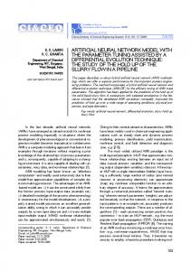
A small Bayesian neural network with ve input units (representing features) and four output units (representing classes). See the text for details.
Figure 1: x1
x2
x3
x4
x5
Features
where sq is the support value of unit q , q is its bias, oi is the output from unit i and wqi the weight from i to q . Now we can identify units in the network with events (both features xi and classes q ), which gives:
q = log(pq ) ! wqi = log ppqip q i sq = log(pqjijk:::)
(5) (6) (7)
If we want the activity of an output unit q to be the posterior probability of the corresponding class, we get an exponential transfer function. Since the independence assumption often is only approximately ful lled, these equations give only an approximation of the probability. Therefore it is also necessary with a threshold in the transfer function, to prevent probability estimations larger than 1: ( 1 sq � 0 (8) �q = exp s otherwise q
The measure �q of the posterior probability of q is also called the belief value of unit q . Thus, in the network there is one unit for each possible feature, and one unit for each class (see gure 1). To use a trained Bayesian neural network, the units corresponding to observed features are stimulated in such a way that their outputs, oi , are set to 1. The activity is then spread through the weights (6) to the output units, which sum their inputs according to (4). This sum, or support value, of each unit is then fed to the transfer function (8), the result of which is returned as an estimation of the posterior probability of the corresponding class.
Feedback connections
There is no real di�erence between the classes and the features in the above deduction. They are just treated as stochastic events. Also note that the weights wqi are symmetric, i. e. wqi = wiq . This suggests that we can use this as a recurrent neural network, similar to the Hop eld model [11]. The probability estimations from the rst step are fed into the next step, and so on until a stable state is reached, i. e. relaxation. This is an important aspect of the Bayesian neural network model, which allows for several useful applications [15]. Relaxation implements a \winners-take-all" operation which causes the network to choose the \most likely" interpretation of the input, among several competing ones. However this will not be further treated here, where we will instead concentrate on the classi er aspect. The fact that each unit is connected to all other units can be utilized without full relaxation. If we let the signals propagate only \one step" through the network (i. e. we do not let the output 2
from the rst step be the input to any further steps), the network will, given some observed events, calculate the posterior probability of all other events. Thus it is possible to use this recurrent, or autoassociative, structure in the network without iterating to a stable state. Above, �q denotes the belief value of the receiving unit and oi the output of the sending unit. Since there is no di�erence between sending and receiving units, we want all units to have the same transfer function. Although a units output oi and belief value �i are not the same things, it is common in this simple version to merge the calculation of them into one transfer function [15]: 8 > si � i exp si i < si < 0 :1 0 � si This equates to the belief value (equation (8)) when the support value is stronger than the bias i, and zero otherwise. Stimulation of the units are put on their inputs, according to a slight adjustment of equation (4), consisting in replacing the bias with an external stimulation �i :
si = �i +
X j
wij oj
(10)
Before we have observed anything about xi , �i = i = log(pi), giving zero activity. After measurement of the event, �i is set to the logarithm of the posterior probability of the event (i. e. of how much we believe in the event after the measurement).
Training of the network
During training of the network the weights and biases are set up according to estimated values of pi and pij from a set of training patterns. This is done via counters in the units and in the weights in the following way:
C = ci = cij =
X �
X �
X �
�(�)
(11)
�(�)�i(�)
(12)
�(�)�i(�)�j(�)
(13)
where � is the pattern number, and �(�) is the strength of pattern � (it amounts to showing that pattern to the network �(�) times). The value �i(�) = P (x(i �)) need not be binary, but can once again be a probability, then interpreted as the proportion in the population described by pattern �, having attribute xi . If more than one attribute in a training pattern has graded probabilities associated to them, this is interpreted as if these probabilities are independent with respect to that pattern. If two such \uncertain" attributes are not independent, then the pattern should be split up in two or more examples of the class (e. g. if the population of q consists mainly of two groups, one with both xi and xj and one with none of them, at least two examples are required to describe this population). Training is done in one pass over the training set, during which the counters are updated for each pattern, according to (11) - (13). Thereafter the real weights and biases are calculated from these counters. The probability of an event is estimated as the number of observations 3
where that event occurred divided by the total number of observations, that is as:
p^i = Cci p^ij = cCij
(14) (15)
Since we are going to take the logarithm of these values, special care has to be taken when some of the counters come out as 0. In practice the logarithm of zero is replaced with a number just slightly more negative than all other values (of biases or weights) in the network. There is no good probabilistic reason for this. On the contrary, if we want the best probabilistic estimation of the distribution over the training patterns, we should use a su�ciently large negative number to make sure that it outweighs all other contributions to a unit. But high accuracy of the distribution in the training set does not guarantee good results of generalization. Just because some situation has not occurred in the training set it does in most practical situations not mean that it is impossible. If the network is stimulated with a pattern not in the training set there is a large chance that all classes have some features in the pattern against them, which would then set all probability estimations to zero. But we still want the least inconsistent alternative to get the highest probability. If su�ciently much speaks for a class, we want this to outweigh the fact that some features are contradictory according to the database. Thus, the more negative a value is chosen instead of log (0), the better the accuracy of the probability estimations gets, but at the same time the generalization capability and fault tolerance in the network will decrease. The following choices are somewhat arbitrary, but has empirically worked well. Weights between units are set to: 80 ci = 0 _ c j = 0 > < log 1 =C c wij = > c C ij = 0 (16) : log c c otherwise ij
i j
and biases to:
(
log 1=C 2 ci = 0 (17) log ci =C otherwise There are also other methods that avoid the problem with zero probability estimations by assuming suitable prior distributions on pi and pij [9].
i =
The independence assumption
To derive the network model above, we had to assume independence between the di�erent features, both unconditionally and conditionally given q :
pijk::: = pi � pj � pk � � � and:
pijk:::jq = pijq � pjjq � pkjq � � �
(18)
(19) Complete independence in this way is of course usually not the case in real situations. (It might be objected that what is assumed is actually that xi ; xj ; xk : : : are in some sense \equally" dependent unconditionally, as when conditionally given q , i. e. for all classes q :
pijk:::jq pijk::: = pi � pj � pk � � � pijq � pjjq � pkjq � � � 4
but even if this might soften the situation somewhat, the exact ful llment of this relation is in practice equally unlikely.) Of the two relations the rst one, (18), is actually often less important than it might seem. Since the error factor from this is independent of q , it yields an equal over- or under-estimation for all classes. This means that if we are only interested in the probability ordering of the classes, this is not a�ected at all. Furthermore, if we want the actual probabilities we can always normalize them over all classes, thus compensating for this error. The second relation, (19), is more important since it directly a�ects the ordering of the classes, which of course is serious in a classi cation system. There is an important special case in which this relation always holds though. It is when we can express each class with one single example, a prototype, possibly with graded values of its attributes. (Remember that the interpretation of graded attributes in a training pattern is that they are independent with respect to that pattern. This follows directly from the way the counters are updated, equation (13).) In the model with feedback connections as above, in which the probability of all unobserved events are estimated from observed events, the analysis gets more complicated. In particular though, if one event tells anything about another they are certainly not independent. This means that in the feedback case, we can never get complete independence between all units (or else the system would be useless anyway, with all weights zero). In spite of the violations of this independence assumption, it actually turns out to work in many situations. One explanation might in part be that di�erent dependencies cancel each other out, or that many of them do not a�ect the ordering of the classes. Important is also that even if all units are not independent, the best we can do is to assume independence, unless we know some extra structure of the problem, or have nearly unlimited amounts of training data. What we would like to do, to get as correct probabilities as possible, is to estimate the entire joint distribution over all events. This can of course be done by introducing \bins" for all combinations of outcomes and counting how many training examples that goes into each bin. When the number of training examples increases, the fraction of examples in each bin goes to the probability of that joint outcome. But if we have n binary events, 2n bins would be needed (the \curse of dimensionality"), and in practice we usually have a very limited amount of training data (and even if we had enough data, we would not have time to wait for the processing of it). This means that most bins will be empty, and we know very little about the distribution there. Instead we have to utilize each training example better (or to reduce the number of freedoms in the problem). To do this we must assume some additional structure of the problem, and if we do not know anything special about the domain, independence between events is the most natural (see also [4]). The gain in generalization from the events for which this assumption is correct, might often outweigh the distortion in the probability from the cases where it does not hold. Still, in many cases there is some other structure of the problem, which makes the independence assumption clearly useless, as in the parity-problem, or when dealing with e. g. translation invariance or other invariances. Even in less extreme situations, this independence assumption is what limits the operation of the one-layer Bayesian neural network most. Therefore we will in section 4 and 5 treat di�erent versions of multi-layer extensions of the model that can help overcoming this limitation.
5
3 Fully covering codes
The above model does not handle situations where we may want to state that something has not occurred. Activity zero of an input unit rather means that we do not know anything about the corresponding feature, since zero activity does not in uence anything in the network. One solution is to add another unit for the negation of the feature. Such a coding can be called a complementary coding [20]. Thus if no observation is done, both units have zero activity and does not a�ect anything in the network. Otherwise the weights from the positive unit corresponds to the change in the network if there is positive evidence for the feature, and the weights from the negative unit the change if there is negative evidence. When complementary coding is used, one would expect the belief values of the positive and negative output units to sum to one. Due to the independence assumptions that are not always ful lled, the sum usually di�ers somewhat from one. One way to compensate for this, is to calculate the belief value (i. e. the estimate of the posterior probability) of the feature as the average of the belief values dictated by the positive and the negative unit: �^i = �i + (12 ? ��i ) (20) The positive and negative evidence for a feature above might be seen as two di�erent outcomes of a random variable. In general we may have any number of mutually exclusive (and exhaustive) outcomes of a variable, and each outcome can be represented by one unit in the network. We call such a coding, with groups of mutually exclusive and exhaustive units (i. e. such that for all patterns, exactly one of the units in each group is active), a fully covering code. Note that this implies even activity in the patterns since exactly one unit in each group is active in each complete pattern. Now we have introduced groups of strongly anticorrelated units, which a�ects the derivation in the previous section. Assume that we have n such independent groups (or variables) Sj , with di�erent outcomes i. Let �q denote the posterior probability of a class (i. e. the probability of q given the observation) and �i the probability of the outcome i after measurement of the corresponding variable (in the case of completely determined input always 0 or 1). Instead of equation (2) we now get:
�q = p q �
Y pqjS j
pq = pq � j
Y Pi2S pqji � �i ! j
pq
j
0 1 Y @ X pqi A = pq � p p �i j
i2S
j
q i
(21)
The next step is to take the logarithm of this equation, to get a sum of the product. But then we would also need to take the logarithm of the sum inside the product of (21), which of course does not give anything simple in general. (Observe that if we just skip the logarithm, we already in (21) have the structure of a pi-sigma network [8].) However, for completely determined input (i. e. in each group exactly one �i is 1 and the rest 0), each sum consists of only one nonzero term. Thus we might take the logarithm of each term separately, and let oi pick out which one to use, where oi = 1 if �i = 1, and oi = 0 otherwise. Thus it is possible to write: log(�q ) = log(pq ) +
X j
0 1 ! X X p p qi qi @ A log �i = log(pq ) + log p p oi q i i i2S pq pi
(22)
j
This is the derivation of the Bayesian model for fully covering codes. As can be seen, the result of this equation is identical to that of (3), which means that the weights and biases are 6
calculated in the same way as before, and the network is used in exactly the same way as the basic model. One important use of this kind of coding is for handling n:ary attributes. Each possible value of the attribute gets one unit in the network. It is equally important though, as we shall see, for handling complex columns (introduced in section 4) and continuous valued attributes (section 6).
Complementary coding and graded input
When we now can treat evidence both for and against a certain event, it would be preferable if graded input, i. e. evidence between absolute certainty in either direction, could be handled. What we would like to input to the network is not only whether an event xi has occurred or not, but more general the posterior probability of the event (i. e. we have made some measurement of the event, but the result is not conclusive). In speci c, we want to be able to state that we do not know anything further for some event (i. e. we have not measured the event at all), and in that case this input must not in uence the activity in the network in either direction. But the reason that equation (22) holds, is that exactly one �i from each Si is one, and the rest zero. Thus the sum over each group consists of only one non-zero term and we can take the logarithm of that element only. If we want to preserve the network structure with units that sum their inputs, the best we can do for other values of �i is to choose oi to provide a piecewise linear approximation of the real logarithm. For the case of exactly two units in each group, i. e. a complementary coding of binary attributes, we want to approximate the in uence from one pair of units fi; �ig on another unit q :
0 1 ! ! X p p p p p �i �i qi qi qi q q log @ p p �i A = log p p �i + p p ��i = log p p �i + p p (1 ? �i ) � � i2S
j
q i
q i
q i
q i
q i
(23)
An example of what this expression might look like is shown in gure 2a. This will be approximated by the following expression, linear in the activities oi and o�i :
!
!
p log ppqip oi + log p qp�i o�i q i q �i
(24)
If we would let oi = �i for continuous �i , this would yield a straight line between the values corresponding to strict binary input. This approximation is usually not very good. If q is positively correlated with xi , then it is negatively correlated with x�i . This means that the logarithm changes sign somewhere between the end points. This change of sign occurs exactly when we do not know anything about xi , and thus �i = pi (the apriori probability). Before we know anything about xi we do not want its pair to in uence anything else in the network, i. e. we want its in uence to pass zero. But the completely linear approximation above do generally not pass zero at that same point, which results in a lot of activity in the network before we have input anything (see gure 2b). But since we have two units it is actually possible to approximate the in uence with two linear pieces, by e. g. letting unit i be active only for �i above pi , and unit �i active below pi . This is actually what is done when transfer function (9) is used. In e�ect this lets oi = �i but thresholded so that only one unit in the pair is active. Unfortunately this yields a discontinuous function, since a unit suddenly goes on when its belief value exceeds pi . This is shown in gure 2c. More natural then is to rescale the output to increase continuously from zero when �i = pi , and up to one when �i = 1. This will normally give a much better 7
1
1
0.5
0.5
0
0.2
0.4
-0.5
πi
0.8
0.6
0
1
0.2
0.4
-0.5
-1
0.6
0.8
1
0.6
0.8
1
-1
a
b
1
1
0.5
0.5
0
πi
0.2
0.4
-0.5
πi
0.8
0.6
0
1
0.2
0.4
-0.5
-1
πi
-1
c
d
Figure 2: The desired support from one complementary pair of units on another unit, and some piecewise linear approximations of it. (a) An example of the support from x to q according to equation (23). The parameters here are p = 0:1, p = 0:2, and p = 0:08. (b) The linear approximation that results if we set o = � in (24). Note that this does not pass zero at the apriori value of � , 0:2. (c) The result of using the transfer function (9), which is zero at � = 0:2 but instead not continuous there. (d) Finally, the approximation suggested by (25), which is both continuous and passes zero at the right place. i
q
i
i
qi
i
i
i
approximation which is both continuous and makes the network quiet before we have stimulated it ( gure 2d). Expressed as a function of �i , oi becomes:
oi =
(
�i � pi pi < �i
0
� ?p 1?p i
i
i
(25)
The new transfer function will be:
8 > < 0 ?exp si � i i < s i < 0 oi = > exp1?s exp :1 0 � si i
i
i
(26)
The posterior probability, or the belief value of the unit, is still estimated as:
�q =
(
1 0 � sq exp sq otherwise 8
(27)
This means that we have to separate the estimation of the posterior probability �i , from the output oi of the unit. Although now the probability is not itself fed out of the network, it can readily be calculated from the output of the units. The new output can be interpreted as the ratio of known positive instances (as opposed to completely unknown), instead of as before the expected ratio of positive instances (as opposed to negative instances). For more than two units in some Sj it is harder to nd a good approximation. A generalization of the above to the case of n non-negative �i summing to 1:0, that yields a piecewise linear approximation of the logarithm, requires a kind of normalization of activities in each group:
kj = min � =p i2S i i oi = �i ? kj pi j
(28)
There are situations in which this approximation is not su�ciently good, which then requires another approach, as discussed in a subsection to the following section.
4 Complex columns
The normal way to treat strong dependencies among the features is to add an intermediate layer between the input (features) and the output (classes) [14, 10]. This intermediate level consists of complex units, i. e. units that combine information from the input layer. If for example the units a and b are correlated, we produce a complex unit ab that is active when both a and b are active. The classes will now depend on a, b and ab, but these three units are certainly neither independent nor mutually exclusive, and the Bayesian model can not be used directly. One way to get independent groups of mutually exclusive units is the following procedure. If we start from a fully covering code, and nd that two groups of events, corresponding to two random variables, are dependent, we merge the two groups into one, with all possible combinations of the outcomes of the old variables. For example, if two groups of units corresponding to primary features A = fa; a�g and B = fb; �bg are not independent, we insert in their place the composite group AB = fab; a�b; �ab; �a�bg. We call this kind of group, with all possible combinations of some primary features, a complex column. If we manage to divide the primary features into independent groups, we can create a complex column from each such group. The Bayesian model is now directly applicable on these complex columns, via equations (21) and (22). In this way the mechanism of complex columns solves the problem of dependence between features. One drawback with complex columns is that the number of units increases exponentially with their order, i. e. with how many primary features they combine. However, it is not necessary to save the units for those combinations which are never used. This will give a considerably lower number of units (if all training patterns are binary). In the extreme case, when all primary features are gathered in the same column, we will get one unit active for each training pattern, i. e. grandmother units. Also compare the architecture described in [21], where the training patterns are given one unit each in the network. Another problem with these complex columns is that when they grow larger, the generalization capability tends to decrease. This is the same trade-o� between probabilistic accuracy and generalization as discussed in section 2 above, and it should prompt us not to unnecessarily raise the order of the columns, but only merge columns whenever it is actually required.
9
q1
AB
_ ab
ab
a
_ a
q2
_ ab
q3
__ ab
b
_ b
q4
Classes
c
_ c
C
c
_ c
Features
Complex Columns
Figure 3: A Bayesian neural network with a complex column layer. The three primary features a, b and c, are grouped into one rst order column C and one second order column AB . Between the complex columns and the output units (here representing classes) are the Bayesian weights.
Selecting complex columns
Still the problem remains of where among the features to create complex columns, i. e. where the correlations are too high. In general it is a very hard problem to nd the independent partition of lowest order (possibly of exponential complexity, but compare the results in [2] and [23]). A partially heuristic method that has shown itself very useful though, is the obvious one of merging two columns whenever some measure of correlation between them is high [14]. For this heuristic method, the hidden layer initially consists of all primary features (complementary coded), which can be considered as complex columns of order one. In the rst pass, second order correlations are detected and removed by merging the corresponding features. Additional passes removes higher order correlations (i. e. pairwise correlations between higher order units) that has become visible by the previous passes. (This method of incrementally creating higher and higher order units is similar to the one described in [12].) One advantage with this method is that the construction of complex columns is unsupervised. An example of a measure that can be used to decide if two columns are to be merged, is the covariance between two units i and j , pij ? pi pj . If this measure exceeds some threshold for any pair of units in two di�erent columns, these columns are merged. Note that once two columns are merged, they may not be separately merged with additional columns, since each primary feature is allowed to contribute to just one complex column. If a column is correlated with more than one other column, it may be merged with only one of them in the same pass. Additional merging of the new column might of course occur in following passes. This method has in tests turned out to very e�ciently reduce the amount of correlation in the network, often su�ciently much after only one or two passes (i. e. at most fourth order columns). Other measures of correlation than the covariance can be advantageous in other kinds of applications [14, 16]. In the case of dependencies that are not detectable from lower order statistics, other approaches has to be used. E�cient methods for nding decorrelating internal representations is currently a focus of our further work, as well as for several other groups [10, 24, 25, 7].
Propagating signals to the complex columns
The structure of the network is now that a hidden layer with complex columns is inserted between the primary feature units and the class units. The rst layer is complementary coded, i. e. each 10
primary feature is represented with two units. Each complex unit has input connections from the primary units it is a combination of. Between these complex columns and the class units is a normal Bayesian neural network (see gure 3). For binary input the activity of a complex unit can be calculated by multiplying the activities of the units it is a combination of. This would also have been a good approximation for the case of graded input (corresponding to �ab = �a �b ), if its primary features would have been independent. But the very reason to create the column is just that they are not independent. The problem now is to estimate the joint probability �ab from the marginals �a and �b , when we know how correlated a and b are. This is actually not as trivial a problem as it might seem from a rst glance. For just two marginals �a and �b , �ab is the solution of a quadratic equation, but for the general case with a higher number of marginals, there is probably no exact closed form solution, although there is an iterative method (the IPPF method, see e. g. [3, 28]). Since we have to make an approximation for graded input anyway in the complex columns, there is no idea to try to get an exact expression in the current situation. It often su�ces if the result is exact for the extremal values of the input and for the apriori values, and gives a reasonable approximation in between. Especially suitable are expressions of the form:
�abc::: � �au �bu �cu � � � b
a
c
(29)
What is nice with this form is that if we take the logarithm of it, the ui 's will become the weights of the input connections, and the complex units will still be just summing their input (and what should be input is anyway the logarithm of the probability). If we set all ui in a column to the same value, and require that the result is exact at the apriori values, i. e. : pabc::: = (papb pc � � �)u then we get for u: log(pabc:::) u = log( (30) pa pb pc � � �) A slight modi cation of this, that di�erentiates the values ui in a column is: log( p pp p ��� ) (31) ui = n log( pi ) + 1 abc:::
a
b
c
where n is the order of the unit (the number of input connections). It also ful lls the above requirements, in that it holds an exact result for binary input and for all input unknown, and can be expected to be slightly better than (30) in between these inputs. Unfortunately it is not possible to get an expression of this form that holds exactly for all combinations of known and unknown primary features in a column. During training (i. e. collecting of the statistics for the p's) all weights ui should be set to 1 (meaning that we assume them independent until we know better), and thereafter changed according to the above equation. In practice the values of ui does not matter during training (as long as they are strictly positive) if we use only binary training patterns, since the result will anyway be either zero or one in that case. But if we want graded input in the examples, remember that the interpretation of this is that the graded attributes are considered independent relative each example, which motivates setting ui to 1 during training in this case. Equations (29) and (31) do not guarantee that the probabilities in a complex column sum to one. This is usually not a big problem, since it is often close to one, and anyway it is always 11
possible to normalize the activity over each column (which has to be done anyway if (28) is used). To propagate the signals down from the columns to the primary feature units again is much easier. This can be done by just adding the belief values of the units in the column that take input from the primary feature, i. e. for example �a = �ab + �a�b . Here too, normalization might be necessary, but this can be done either before or after the addition. If it is done after, only two units are involved in each feature, which makes this normalization more \local".
A better approximation for graded input
The above constructions give the correct result for the probability estimation when all primary features in a complex column are known, and also when all the input to a column are at their apriori values (i. e. unknown). For intermediate knowledge, either such that some of the primary features are known and the rest completely unknown or that all or some primary features have graded input probabilities, it will yield only an approximation. Often this approximation will do, but in some special cases it is not good enough. This occurs when some of the units in the column are strongly anticorrelated to a receiving unit, and thus has very large negative weights to that unit. Even a very small activity in such a complex unit will suppress the activity in the receiving unit, much more than it ought to be suppressed according to the middle expression of equation (22). This is due to the linearisation of the logarithm in the right of (22). Let us look at an example of what e�ect this may have. Suppose that we have a complex column fab; a�b; a�b; �a�bg, and among others two classes q and r. If we know a but not b, then both ab and a�b will get slightly active. Suppose now that q always is associated with ab, and r always with a�b. Then both q and r should actually get slightly higher probabilities (relative all other classes), since their respective symptoms has got higher probability. But what happens is instead that ab suppresses r strongly, since they have never occurred together, and a�b suppresses q, and both q and r get decreased activity. One way to make the approximation much better is to add units for \don't know" in the groups corresponding to primary features, fa; ao; a�g, and combine these into the complex columns too. (The idea to handle \unknown" values explicitly is also used by others, e. g. [6].) This means that the size of a complex column will increase as 3n with the number of primary features, instead of as 2n . Still inhibition might get too strong, but the result will now be exact on considerably more points, and thus more accurate in between too. Further, what is more important is that no two completely incompatible units will be active at the same time, suppressing each others e�ects. For our example above it means that only the unit for abo will be active, which supports both q and r with the correct strengths. If then some slight evidence for b turns up, ab will begin to get active, suppressing r but supporting q, which is just the behavior we want. If this kind of complex columns are used, equation (29) is not needed to propagate the signals up to the columns, since the activity will anyway get correct when all (or some) primary features are unknown. Therefore normal multiplication will be su�ciently good. By the same reason the normalization (28) is not appropriate for this case. During training all \don't know"-units have to be active, meaning that even if an object has an attribute, this attribute might pass unobserved. During recall they are active to the extent that their attributes really are unknown.
12
a1 _ _
a2
a3
a4
_
b1
ab11 pa1b1 pa2pb1 pa3pb1 pa4pb1
b2
pa1pb2 pa2pb2 pa3pb2 pa4pb2
B
_
A
b3
ab pa1pb3 p 23 pa3pb3 pa4pb3 a2b3
b4
pa1pb4 pa2pb4 pa3pb4 pa4pb4
A fragmented column AB with only two units, ab11 and ab23 . For all other cases the approximation P (a b ) � P (a )P (b ) is su�ciently good, and we can thus use the activities in the columns A and B separately. If any of the units in the fragmented column goes active, it has to inhibit its corresponding units in A and B to ensure that we have activity in either A and B , or in AB only.
Figure 4:
i j
AB
Fragmented columns
i
j
The way complex columns are created up to now, is to merge two smaller complex columns whenever some unit in one of them is too correlated with one unit in the other. If the two columns are already quite big, we will get a very large number of new units, although perhaps only one pair of original units were signi cantly correlated. As before this may impair the generalization in the network, when we have a limited amount of training data. In such situations it might be tempting to give up the column idea, and merge separate units instead of entire columns. It is nothing wrong in that as long as the resulting units get more uncorrelated, but this has to be done very carefully, not to introduce additional correlations instead. Fortunately there is no need to leave the column idea altogether. Suppose that we have two relatively large columns A and B , and suppose that the units inside them are mainly uncorrelated between the columns, such that P (ai bj ) � P (ai )P (bj ). This means that we get good results even if the columns A and B are kept separated. But if now for one speci c a 2 A and one speci c b 2 B this is not ful lled, a complex unit ab would be needed to give a better result for this case. Thus there seems to be two distinct alternatives for the two columns A and B . Either we merge them to AB , and the result will be good for the case ab, but we will have a large number of units which requires more training data to estimate the densities reliably for, or we let A and B be separated, and the results will be all right for the other cases ai bj but bad for ab. The solution is to use fragmented columns. Suppose that we in only the case ab use the corresponding unit from the column AB , and for all other cases uses the units from A and B separately. Then we will get the good things from both alternatives (see gure 4). In general, if we have di�erent alternatives of how to create complex columns, we can use fragments from each alternative if we make sure that only units from one alternative are active at one time. In the case of our example, it can be done by letting the unit ab inhibit unit a in A and unit b in B. If graded input is to be handled by this kind of model, the inhibition should subtract the activity of ab from both a and b. In general it might require some thought to nd out which units have to inhibit which, speci cally when these column fragments are to be merged with yet another (possibly fragmented) column. This will add quite an amount of administration on top of the network.
13
5 Multiple covering
In equation (21) it is assumed that each primary feature occurs in only one complex column. If some primary feature is a member of more than one column, these will not be independent. If e. g. A is a member of the columns AB and AC , A will leave its contribution to two di�erent factors of equation (21), which will distort the estimation of probabilities in the Bayesian model. This is of course a limitation. If A and B are dependent, as well as A and C , but B and C are not signi cantly dependent, then this means that we would still need to make a column ABC . (The fragmented columns above are not guaranteed to help in this situation.) Since this is of a higher order than having two two-order columns, and it consumes considerably more memory, this can be a serious problem in some applications. Thus in many situations it would be more convenient if the columns were allowed to overlap. An important special case where such overlap occurs is a higher order network [22, 1]. In e. g. a second order network all second order events are represented, which in terms of this model means that we have one column for each possible pair of primary features. Still higher orders are de ned similarly. These higher order networks can be considered as compromises ranging from the complete independence assumption, assuming more and more dependence, and nally estimating all outcomes of the joint distribution separately. If we only have rst order units in the network, the best we can do is to assume independence. If we have all second order units, this will give a better approximation, and so on. The problem is to estimate the joint probability pijk::: given the marginal distributions of some order (or possibly marginal distributions of di�erent orders). If we only know all rst order marginals pi , pj , pk : : : the \best" estimation is:
pijk::: � pi � pj � pk � � �
(32)
which is the usual equation for independent marginals. To get the best estimation when we know all second order marginals pij , or for any higher order is not equally easy. There is no closed form expression, but only an iterative method (the same IPPF method as mentioned above, [3, 28]). Although this iterative method is quite simple, and often converges quite fast, we would rather like a closed form approximation. There are a few alternatives, but here we will consider two, that are specially suitable for implementation in this kind of neural network. The rst approximation is suitable when all primary features occur in the same number of complex columns, as is the case with higher order networks. If we consider a second order network with n primary features, each of them occurring together with n ? 1 others, then the approximation used is: pijk::: � ?ppij � pik � pjk � � � (33) If all events are independent, this will give the same result as (32). If there are some pairwise dependencies, the product will be adjusted in the correct direction, and thus making a better approximation than (32). For the Bayesian neural network, equation (21) is changed to: n
1
?ppij jq � pikjq � pjkjq � � � Y ?s pijq pijk:::jq pqjijk::: = pq � p � pq � ?pp � p � p � � � = pq � pij pq ijk::: ij ik jk i;j 2P n
1
n
n
1
1
(34)
In general, if each primary feature occurs in m complex columns (an m-covering code), we can compensate for this by taking the m:th root. It can be seen as calculating the probability given each of the m coverings separately, and then taking the geometric average of them. This 14
amounts in the weights (i. e. after taking the logarithm) to a division by m. Otherwise the Bayesian model is exactly as before. The approximation (33) usually underestimates the real e�ect of the second order dependencies. A more rigorous approach is to try to express the joint probability distribution as a series expansion in higher and higher order marginals [5]. Especially suitable for the Bayesian model is a product expansion, since taking the logarithm will transform this into a sum. Similar product expansions to the one used here, are treated in e. g. [17] and [28]. We propose the following form of expansion:
P (X ) =
Y i
1 (xi )
Y ij
2 (xi ; xj )
Y ijk
3 (xi ; xj ; xk ) � � �
1 (xi ) = P (xi ) 2 (xi ; xj ) = PP(x(x)iP; x(xj ) ) i j P ( x ; x ; x 3 (xi ; xj ; xk ) = P (xi ; xj )Pk )(Px(;xxi )P)P(x(xj )P; x(x)k ) i j i k j k .. . Y m (S ) = P (R)((?1)j j?j j ) S
R
R�S
(35)
(36)
where S is a set of size m of variables xi called the support of m (not to confuse with the support value of a unit), and R goes over all (nonzero) subsets of S . The exponent (?1)jS j?jRj controls whether the factor goes to the numerator or denominator (for odd di�erences jS j ? jRj it goes to the denominator). Each m can be seen as making a correction to the product of all of lower order with support from a subset of the support of m . Actually, an alternative way of writing (36) is in a recursive form: (S ) = Q P (S () R) (37) R�S
where we have dropped the index of that speci es its order. The idea is to truncate the higher order terms of (35), to get a lower order approximation of the distribution. One possibility is to truncate all m above a certain order. If we for example include all second order statistics and simplify, this yields the approximation: Y Y (38) pijk::: � P (xi) PP(x(x)iP; x(xj ) ) = (ppij� p� pik� p� p�jk� �)�n�?� 2 i j i j k i ij Note that if one xi 2 S is completely independent of the other variables in S , then m (S ) = 1, and will not a�ect the product. Also note that a certain m (S ) cancels out all lower order (R) with R � S from the product, leaving only the factor P (S ). These two facts together imply that if there is a partition of the primary features into independent groups of size � m, then an expansion with all terms up to order m (or higher order) gives an exact result. But it is not necessary to include all factors up to some order. It is possible to mix the orders, which leads us into a larger and more important class of situations in which an expansion like this gives an exact result. All distributions P (X ) can be written as:
P (x1 ; : : :; xn) = P (x1)P (x2 j x1)P (x3 j x1; x2) � � � P (xn j x1; : : :; xn?1 ) 15
(39)
Suppose now that the variables can be ordered such that each variable depends only on a few of the preceding variables. This means that they can be ordered in a directed acyclic causal graph. Say that no variable depends directly on more than m other variables. Then there exists a product expansion with factors from (35) of no higher order than m +1, that gives the desired distribution. This is because each factor that introduces a new variable looks like P (xi j S ) where S is a set of at most m variables, and xi has not occurred in any earlier factors. This factor can be written: Y P (xi j S ) = PP(x(iS; )S ) = (xi; R) (40) R�S
(this time R is also allowed to be the empty set. If uncertainty occurs as to whether the empty set is to be included, just include it and let P (fg) = 1). Thus for each new factor we add the right hand side of this equation, where no factor depends on more than m + 1 variables. In practice it might be unusual that the primary features can be partitioned into completely independent groups, of su�ciently small size. But it is much more likely in technical and other systems that although all primary features might be dependent on each other, they have some direct causal relation to just a few of the others. This mechanism is in such situations the one needed to actually remove the limitations otherwise imposed by the independence assumption. Before writing out what this means for the neural network, let us note a useful relation. By (S j q ) we denote the product corresponding to (S ) but with all probabilities conditioned by q: Y Y (41) m (S j q ) = P (R j q)((?1)j j?j j ) = P (R; q)((?1)j j?j j ) S
S
R
R
R�S
R�S
where the last equality follows by multiplying by P (q ) equally many times in the numerator and the denominator. With the help of this we observe: Y (S; q ) = P (R)((?1) j j ?j j ) (
S
+1)
R
R�(S [fqg)
0 10 1 Y Y j j ?j j j j ? j j )A @ P (R; q )((?1) )A = @ P (R)((?1) R�S R�S 0 1?1 0 1 Y Y = @ P (R)((?1)j j?j j ) A @ P (R j q )((?1)j j?j j ) A = (S j q ) (
S
S
+1)
(
R
R
S
S
R�S
R�S
+1) (
R
R
+1)
(S )
(42)
Now, let us assume that we have the same causal structure on the features unconditionally as conditionally given q (we can always choose the union of the two causal structures, if they di�er), which means that pijk::: and pijk:::jq can be expressed with the \same" factors, although for the latter they are conditioned by q : Y pijk::: = (Sl )
pijk:::jq =
Yl l
(Sl j q )
Then we are ready to write down the expression we want the network to calculate: Q (S j q) Y pijk:::jq = pq Ql (lS ) = pq (Sl ; q ) pqjijk::: = pq p ijk::: l l l 16
(43)
Each Sl is a set of variables with di�erent outcomes. Thus each Sl actually corresponds to a complex column, with units for all possible outcomes of the variables in this set, and each outcome has of course its own probability and . Let sl be a speci c outcome of the variables in one of these sets, and thus let l run over all sets and all outcomes in each set. The result of taking the logarithm (and assuming binary input) is then: X log(�q ) = log(pq ) + log( (sl ; q ))ol (44) l
where ol = 1 if all outcomes of primary features of the complex unit l are in accordance with sl . The bias and the support value of the units are as before, but what has changed is the formula for the weights from units in the complex layer: wql = log( (sl; q)) (45) Note that the weights are symmetrical, in the respect that they only depend on which events are involved, not from which or to which. Also note that in the case where Sl consists of only one variable, this weight will be the same as in the basic model. There is a heuristic method for constructing multiple coverings like this. It is similar to the way the normal complex columns are constructed. Just as in that case, the method is not guaranteed to nd and compensate for all correlations, but in many situations it can be expected to work. First we impose a restriction on the form of the product expansion. For each factor (S ) that is included, also all factors (R) with R � S must be included in the product. This will simplify the administration a lot, without a�ecting the result too much (since it is almost always what we want to do anyway; compare equation (40)). Just as in the case of normal complex columns, the hidden layer initially consists of complex columns of order one, corresponding to all primary features. Thereafter for each pair of complex columns which are too largely correlated, a new complex column is created from their combination. What is di�erent here, is that the two original columns are not removed when we create a new column. Also the same primary feature might be a member in more than one higher order column. This kind of multiple covering is a new and promising aspect of the Bayesian model, and can be expected to work well in many situations where the normal complex columns have problems, due to a large number of units and the bad generalization that usually follows. Of course the number of units in the version discussed in this section, also increases exponentially with the order of the columns, but the whole point of introducing multiple covering is to reduce the required order of the columns. In many practical situations it might be enough with columns of order two or three. Still much remains to do with respect to multiple covering. The details of how to e. g. use it in a recurrent network, handle graded inputs, or get back from a multiple covering to probabilities of primary features are not yet completely worked out.
6 Continuous valued attributes
Up to now we have only treated binary features. Either an object has an attribute or not. When graded input occurs, it is as a probability for the binary feature. But in many situations the evidence we want the network to handle comes from a measurement with a result in some continuous interval. The same mechanism that allows complex columns in the Bayesian neural network model, can also be used to handle continuous valued attributes. The idea is to transform the continuous 17
1
1
0.8
0.8
0.6
0.6
0.4
0.4
0.2
0.2
00
1
2
3
4
5
00
6
1
a
2
3
4
5
6
b
Two examples of sets of base functions P (z j v ) covering the interval [1; 5]. (a) A set of Gaussian base functions. (b) A set of piecewise linear peaks, that will give a piecewise linear approximation of the distribution P (z ).
Figure 5:
i
variable into a number of discrete variables, that can be used directly by the Bayesian network. This is done via a nite mixture of density functions [26, 27]. The probability density function over some continuous variable z can be approximated by a nite sum (although it is a density function, it will be denoted by P (z )):
P (z) =
n X i=1
P (vi )P (z j vi )
(46)
This can be seen as a partition of P (z ) into n subdistributions P (z j vi ), each with probability P (vi ) of being the \source" of z (expressed in another way, random numbers with the distribution P (z) can be generated by rst selecting among the subdistributions with probabilities P (vi ), and thereafter generating the number from the selected distribution P (z j vi )). This partition also de nes functions from the value z to the probability of this z being generated from the component vi : (47) P (vi j z) = P (z jPv(iz))P (vi ) / P (z j vi )P (vi )
where instead of keeping track of P (z ), we can use normalization over i of the right hand side, since: n X P (vi j z) = 1 i=1
If each base function P (z j vi ) has a single peak, and decreases monotonically on both sides from this peak (like in gure 5), the transformation can be seen as a kind of soft interval coding. This is the structure assumed here, but most of the equations below hold for other choices of base functions too. Of course it is also possible to let the base functions work on a multi-dimensional z instead of a one-dimensional variable. If the base functions are chosen \close enough", we may assume that this coding preserves the information in the original value of z , i. e. that q depends only on z through the values of vi : P (q j vi; z) = P (q j vi ) (48) 18
This also implies that z only depends on q through vi : vi) P (q j v ; z) = P (z; vi) P (q j v ) = P (z j v ) (49) P (z j vi ; q) = PP ((z; i i i q; vi) P (q; vi) With the help of (48) we come to the key relation in this context; how to calculate the probability of a class given z with help of the base functions P (vi j z ): X X X P (q j z) = P (q j vi ; z)P (vi j z) = P (q j vi )P (vi j z) = P (q) PP(q()q;Pv(iv) ) P (vi j z) (50) i i i i This is easily generalized to the case of a set of independent continuous variables zj : Y X P (q; vji) Y P (vji j zj ) P (q j z) = P (q) P (Pq(jq)zj ) = P (q) j i P (q )P (vji ) j
(51)
Just as in the other cases above, what is treated by the network is the logarithm of this, and just as before the logarithm of the sum is approximated with an expression linear in the activity of units, corresponding to the probabilities P (vi j z ):
! X P (q; vji) P (vji j zj ) log(P (q j z)) = log(P (q )) + log j i P (q )P (vji ) ! X P ( q; v ) ji � log(P (q)) + log P (q)P (v ) P (vji j zj ) X
ji
ji
(52)
For this approximation to work at all, some conditions has to be ful lled. First the functions P (vji j zj ) must sum to 1 for each variable zj , which they actually already do. Next, the expression is exact when one of the P (vji j zj ) is 1 and the rest is zero, so it is preferable if this situation occurs for each P (vji j zj ) at some value of zj , and if only a few (two or three) of the base functions are nonzero in between these values. If for example we use the base functions in gure 5b we get an approximation that ts at the peaks of the base functions, and is an interpolation in between. Finally, if the base functions are placed su�ciently \close" or the probability distribution changes slowly enough, the expression above can be expected to give good values. But we can in this way not only calculate the probability of the classes or other discrete attributes, given the continuous variable. It is also possible to get back to a continuous value from the probability of the di�erent base functions, P (vi ). Since this representation is in terms of a whole distribution, and we want a single value out, it is reasonable to use the expectancy of z : n n X X (53) E (z) = E (z j vi )P (vi) = �iP (vi ) i=1
i=1
where �i is the expectancy of the base function P (z j vi ) (or its mean value). If the base function is symmetric with a single peak, this �i will be exactly at the peak. Now we can calculate the expectancy of another continuous variable y given z . Let y have the base functions P (y j uj ) with expectancy (or peak at) �j , and we have analogously to (50):
E (y j z) =
X j
�j P (uj j z) =
X j
! X P (uj vi) �j P (uj ) P (u )P (v ) P (vi j z) i
19
j
i
(54)
Of course this also generalizes to the case of a set of variables z. Thus when using the network, the values of known continuous variables are rst propagated up to a layer with units whose activity represent the values P (vji j zj ). This layer is fully connected (and has also connections to the class units), and propagating the activity through it calculates the probabilities of uji given the known variables. These probabilities can then be propagated down to continuous values y again, according to (53).
Training with continuous attributes
Still it remains how to train the network with these continuous attributes. One aspect of this is how to estimate the parameters of a number of base functions, e. g. mean value and variance of Gaussian curves, such that they t the distribution in the data as good as possible [26, 27]. Here we will not consider the parameters of the base functions, but instead assume that a set of base functions is selected initially for each continuous variable. They can be placed either on equal distances from each other, or according to a histogram of the data. As mentioned above the mixture will t the distribution better if it has a large number of base functions, but on the other hand, for limited amounts of data the estimation will be more uncertain with many base functions. We may not choose the base functions more dense than that su�ciently many training examples contributes to each of them. Suppose that we have xed a set of base functions P (z j vi ). Then we let e. g. a rst layer in the network transform the value of z through the base function and according to equation (47), or written as (we will not care here about the details of how this transformation is calculated by the network): P (vi j z) = Normalizei (P (z j vi )P (vi )) (55) The value of P (vi j z ) (or the logarithm of it) is fed into the Bayesian part of the neural network. The problem is that to calculate this value we have to know P (vi ), which we don't before training. To estimate P (vi ) directly from P (z j vi ) is not as straightforward as one could hope. There are at least two ways to get around this problem. The rst strategy is to instead x the set of functions P (vi j z ) and let the functions P (z j vi ) be only implicitly de ned from these (since P (z j vi ) will not be needed explicitly anyway). Then we have the following relation, which can be used directly:
Z
P (vi ) = P (z)P (vi j z)
(56)
z
It can be estimated by calculating the sum of P (vi j z ) over all training patterns, and divide by the total number of patterns, which is the way the Bayesian learning rule works already according to equations (12) and (14) (We consider here all patterns as equally \strong", i. e. with � = 1, and thus also C = n. This can be done without loss of generality, since an interpretation of � is anyway just as how many times a pattern has occurred). To see this assume that n training examples with z as an attribute are generated according to the distribution P (z ). Also, as an intermediate step, assume that the interval of z is divided in small bins with width �, and that we calculate separately how many examples that fall in each bin. Clearly we then have: P Z (�) X 0 lim � P (vi j z ) = lim P (v j z 0 ) nz = P (v j z )P (z ) (57) n!1
n
n!1 0 �!0 z
i
n
z
i
where � is the index of the pattern, n is the total number of patterns, and nz0 is the number of examples that fall in the bin z 0 . 20
For the estimation of P (q; vi) we have to, besides (48), make another assumption, which says that all information about vi is contained in z :
P (vi j z; q) = P (vi j z)
(58)
This is more questionable than (48). Actually it is usually not ful lled, unless the probability of q is nearly constant over the interval of support of the base function. Of course this means as before that it can still be made arbitrarily accurate, by choosing the base functions close enough, and if the distribution does not change too fast, it is usually su�ciently good. Anyway, using (58) it is possible to get:
Z
Z
Z
P (q; vi) = P (q; vi ; z) = P (vi j q; z)P (q; z) = P (q; z)P (vi j z) z
z
z
(59)
This is then used to set the weights between the base function units and the class units (or other binary units). Just like above this is what is estimated already, if we use (13) and (15) for training:
P P (v j z(�))P (q(�)) Z X 0 n i qz � 0 = nlim nlim !1 !1 P (vi j z ) n = z P (vi j z )P (q; z ) n �!0 z0
(60)
where P (q (�) ) is 1 if example � is of the class q , and 0 if it is not. Again using (58), i. e. that all information about uj are contained in y and all information about vi in z , we also get the expression for P (uj vi ), which is required for calculation of weights between the base function units of di�erent continuous attributes:
P (uj ; vi) = =
Z
Zyz yz
P (uj ; vi; y; z) =
Z
yz
P (uj j vi ; y; z)P (vi; y; z)
P (uj j y)P (vi j z; y)P (z; y) =
Z
yz
P (y; z)P (uj j y)P (vi j z)
(61)
This is also estimated in exactly the same way, with (13) and (15):
P P (u j y(�))P (v j z(�)) X j i � 0 )P (vi j z 0 ) ny0 z0 = lim P ( u j y lim j n!1 n!1 0 0 n n Z�!0 y z = P (uj j y)P (vi j z)P (y; z) yz
(62)
As conclusion for this way of training the network can be said, that it requires no extra layer in the network to transform the values from the base functions to the input to the Bayesian part of the network, and it requires no change in the training strategies of the Bayesian model. On the other hand, for a xed set of base functions, the estimations of P (q; vi) and P (uj ; vi) does not converge to their correct values as the number of training patterns goes to in nity. But if the base functions are made more dense, as the training set gets larger, the estimations will converge to their correct values, and anyway the e�ect of the approximation is primarily a \softening", or smearing, of the real density, which can actually be an advantage when there is a limited amount of training data (see the example in gure 7 below). Another possible drawback is that there is no simple way of nding the values for �i , since the functions P (z j vi ) are not known. But if the expectancy, alternatively the peak, of P (vi j z ) is used instead, this value will also converge to its correct value as the base functions are made 21
1.5
1.5
1
1
0.5
0.5
00
1
2
3
4
5
00
6
-0.5
1
2
3
4
5
6
-0.5
a
b
(a) A dual set of base functions to the set in gure 5b. (b) One of the duals singled out, to show more lucidly what they look like. Note that there is not a unique set of dual functions for a given nite set of base functions. Also note that all duals to a set of positive functions (with overlapping supports) are negative somewhere.
Figure 6:
more dense. Thus on the whole this method ts naturally into the Bayesian model and can be expected to work very well in practice. But it can also be done in another way, if this approximation is considered as a problem. As opposed to the above, start with a set of P (z j vi ) and consider this as the base functions. To estimate P (vi ) with (56) (or rather with (57)) we have to know P (vi j z ), but to calculate this as in (55) we need P (vi ) rst. Thus (56) can not be used for this. Let us instead introduce the dual basis of P (z j vi ), P � (z j vi ) de ned by the relation:
Z
z
P � (z j vi)P (z j vj ) = �ij
(63)
(where �ij = 0 for i 6= j and �ij = 1 for i = j ). A set of dual functions can be found from the set of base functions without any knowledge about the actual distribution we want to estimate. For example, a set of dual functions to the base functions in gure 5b is shown in gure 6. Note that the functions in the dual basis must be negative somewhere, if the original base functions have overlapping intervals of support. Thus the functions in the dual basis have nothing directly to do with probabilities. Instead of equation (56) we now have the relation:
Z
P (vi ) = P (z)P � (z j vi )
(64)
z
This is easily seen, by inserting (46), and applying the de nition for the duals (63):
Z
z
P � (z j vi)P (z) = =
Z
X
P � (z j vi )
P (vj )P (z j vj ) j Z X X P (vj ) P � (z j vi)P (z j vj ) = P (vj )�ij z j j z
= P (vi )
(65)
Analogously we have for the weights between a continuous attribute and a class:
Z
P (q; vi) = P (q; z)P �(z j vi ) z
22
(66)
This can be seen by rst using (49) to get:
X
P (q; z) =
i
P (z; q; vi) =
and then using this:
Z
z
P � (z j vi )P (q; z) = =
Z z
i
P (q; vi)P (z j q; vi) =
P � (z j vi )
X j
X
X
Z
j
X i
P (q; vi )P (z j vi )
(67)
P (q; vj )P (z j vj )
P (q; vj ) P � (z j vi)P (z j vj ) = z
X j
P (q; vj )�ij = P (q; vi ) (68)
And nally for the estimation of weights between di�erent continuous attributes:
P (uj ; vi ) =
Z
yz
P (y; z)P �(y j uj )P � (z j vi )
(69)
To get this we have to rst use (49) several times to get the relation:
P (y; z) = =
X ij
X ij
P (y; z; uj ; vi) =
yz
ij
P (y j z; uj ; vi)P (z; uj ; vi)
P (y j uj )P (z j uj ; vi )P (uj ; vi) =
And nally using this:
Z
X
P � (y j uj )P �(z j vi )P (y; z) = = =
Z yz
X kl X kl
X ij
P (uj ; vi )P (y j uj )P (z j vi )
P � (y j uj )P � (z j vi )
Z
X kl
(70)
P (ul ; vk )P (y j ul )P (z j vk )
Z
P (ul; vk ) P � (y j uj )P (y j ul ) P � (z j vi )P (z j vk ) y
P (ul; vk )�jl �ik = P (uj ; vi)
z
(71)
This means for the network that we use the dual base functions during training, i. e. while gathering statistics over the training patterns. During recall we use the functions P (vi j z ) calculated from the base functions according to (55), since after training we know P (vi ). This is a more complicated scheme than the previous method, but it converges to optimal values of the parameters when the number of training patterns increases. A comparison of what the two di�erent ways to train the network leads to (for su�ciently many training patterns) is shown in gure 7. The estimation in c is constantly too low in the peaks and too high in the valleys. The deviation in d is much smaller (note that the estimation is only fair in the interval [1; 5] which is su�ciently covered by the base functions). Otherwise the di�erence between the two methods is not very big. Because the dual functions are partially negative, they can give rise to estimations which are also partially negative, and thus not proper probability functions. These negative values of the estimation, of course have to be truncated away. In some sense this negativity of the dual functions means that when training is done with the dual functions we do not utilize the data as e�ciently as with the previous method, since sometimes the counters are increased and sometimes decreased, causing noise to have a larger e�ect. For the limited amount of training patterns that is usually the case, this means that the 23
-4
0.25
1
0.2
0.8
0.15
0.6
0.1
0.4
0.05
0.2
-2
00
2
4
8
6
00
10
1
2
a 1
0.8
0.8
0.6
0.6
0.4
0.4
0.2
0.2 1
2
3
4
5
6
4
5
6
b
1
00
3
4
00
6
5
c
1
2
3
d
This is an example of a distribution, and what the estimations of it done by the network will converge to, when the two di�erent training methods are used. (a) An example distribution P (z ) over a continuous variable z (solid line) together with a joint distribution P (q; z ) where q is interpreted as a class (dashed line). (b) The corresponding conditioned probability of the class, P (q j z ), which we want the network to approximate. (c) What the estimation will converge to, if training is done with the rst method. The base functions P (v j z ) are chosen as the set in gure 5b, and then used during both training and recall. (d) Here is instead the other method used. Again the base functions are chosen as the set in gure 5b but now representing P (z j v ). Training is done with the corresponding dual set in gure 6a, and during recall the functions P (v j z ) derived in equation (55) is used. The constant output at each side is caused by the normalization in (55), since below z = 1 or above z = 5 only one base function has any activity, and normalization will cause the corresponding unit to have constant activity = 1. For both training methods the estimation is only fair in the interval [1; 5], which is su�ciently covered by the base functions.
Figure 7:
i
i
i
convergence to the optimal estimation is slower, and we might have to use the rst method of training instead. Since the approximation in that method results in a smearing of the distribution, this might actually also be an advantage for small data sets, since it reduces the e�ect of noise. Thus, although the second method might be formally more correct, we might in practice have to use the rst method, since it is more straight forward to implement (just one transfer function involved), and can be expected to converge faster to a reasonable estimation.
24
a1
a2
a1
a3
a2
a3
_ b
b
q1
E(z)
b
v1
v2
v3
v4
q1
q2
q3
q2
q3 Output
_
a1b
_
a1b
a1
a2b
a2
a
a2b
a3
_
a3b
a3b
_ b
b
v1
v2
v3
v4
Complex Columns
v1
v2
v3
v4
Input
b
z
Figure 8: This network takes as input three attributes: one ternary, a, one binary b and one continuous attribute, z , coded with four base functions v . The ternary and binary attributes are combined into one complex column (multiple covering is not used here). In the output layer are three class units q as well as copies of all input units. This makes it possible for the network to calculate not only the probabilities of the classes, but also the probability of a primary feature (or expectancy of it in the case of a continuous variable) given some other primary features (e. g. P (a j z ) or E (z j a; b)). See the text for further details. i
j
7 Putting the pieces together
We have discussed the Bayesian neural network model for binary attributes, n:ary attributes, complex columns of di�erent kinds, and nally continuous attributes. In this section we will try to put these di�erent parts in relation to each other, and see how they can be combined in the same neural network. The di�erent kinds of attributes that are treated here are binary, n:ary, and continuous attributes. They are all handled by coding them as discrete sets Si of mutually exclusive (and exhaustive) events (although possibly more than one with nonzero probability). Each of these events gets one unit in the input layer. Thus a binary attribute is coded complementary, i. e. with one unit that is active if the attribute is true and one unit that is active if the attribute is false. An n:ary attribute is coded with one unit for each possible outcome, and a continuous attribute with one unit for each in a set of base functions of the attribute. This is illustrated in gure 8. Exactly how this recoding of the attributes is achieved in the network is not treated here. It can be done either as a preprocessing step before feeding it into the network, or as an additional layer immediately before the usual input layer. In the latter case it is probably most convenient to let the units for a continuous attribute have nonmonotonic transfer functions, corresponding to the base functions, but there are other methods as well. Since all attributes are represented in the same way, they can easily be combined in the same neural network. If the attributes are independent we can just write:
�q = p q �
Y pqjS
25
j
pq
j
(72)
where each Sj can be an attribute of any of the above types. How to calculate the individual pqjS is shown in the corresponding sections above, and turns out to be the same for the di�erent attributes, i. e. just di�erent applications of equation (21). The attributes are of course usually not completely independent. Therefore we have in the layer above the input layer, a complex column layer. If the complex columns of section 4 are used, the idea is to partition the attributes into groups, such that attributes from di�erent groups are independent. Then the attributes in each group can be combined into one joint random variable Sk0 , with units for all outcomes of that variable. Now (72) can be used directly on these Sk0 instead. When two (or more) continuous attributes are combined into a column, this is equivalent to using base functions over a two (or higher) dimensional space (where each complex unit corresponds to one such base function). If both continuous and discrete attributes are combined, the complex units can again be considered as a special case of base functions, over this set of both continuous and discrete variables. A complex unit is active when the input units from which it is a combination, are all active. For graded input the stimuli of a complex unit should be the logarithm of a product of belief values, of the corresponding input units, possibly of the form (29). This can be achieved by letting the activity of the input units be the logarithm of their belief values, and having weights up to a complex unit from all units in the input layer it combines. These weights can either be xed at 1, or if (29) is used, adjusted according to (31) after the training phase. If the kind of multiple covering in section 5 is used, the construction of complex columns is similar. What is di�erent now is that in the complex layer the lower order columns are not removed when they are merged into higher order columns. This means that the higher order columns do not replace the lower order columns, but are instead considered as correction terms for them. The major di�erence from the normal complex columns is in how the weights from complex units in the Bayesian layer are calculated, equation (45). It is between the complex columns and the class units (or output units in general) that we have the Bayesian weights. If we want feedback connections, or use the network as a recurrent network, then there are also connections between the complex columns. After the activities from the stimulated input units have propagated up to the complex columns, it is propagated one step between the complex columns, and then down again through the weights to the input layer. The posterior probabilities of unobserved features can then be read o� from the \input layer". But since this procedure would require slightly di�erent transfer functions for the units when the signals propagate down from the complex columns, than when they propagate up, it might be more convenient to instead duplicate the units from the input layer to the output layer, and directly use Bayesian weights from the complex columns to the copies in the output layer. The class units in the output layer can either be considered as di�erent outcomes of one single random variable, or as separate binary variables. In the rst case they get one unit per class, in the second case each class is complementary coded. This latter case may be advantageous in domains where multiple classes may be active at the same time, as e. g. in diagnoses of diseases, where a person might have more than one disease. In general the units in the output layer may belong to attributes of any of the above kinds, as for example if the some of the inputs units are duplicated in the output layer. To interpret the activity of units from binary or continuous attributes some postprocessing is also needed. For a complementary coded binary attribute the probability is calculated by averaging over the two units, with equation (20). For continuous valued attributes the expectancy can be calculated with (53). This postprocessing can optionally be done in an additional postprocessing layer in the network. j
26
It may often be preferable not to convert an n:ary attribute to a single number, corresponding to the outcome with highest probability, since valuable information is contained in how large the probability is, which alternatives are next best, and so on. Possibly a normalization of activities over the units in the attribute is required, to compensate for approximation e�ects in the network that makes the sum of activities otherwise di�er from 1.
8 Discussion
The aim of this report has been to show that it is possible to extend the Bayesian model to a very general multi-layer neural network that can handle both discrete and continuous attributes. But still much remains to be done with this model. One general complication with complex columns, is that there may be several outcomes with probability > 0 in one column. Then a linear approximation of the logarithm is done, which might be a very bad approximation if the probability distributions change to much between \adjacent outcomes". Therefore it might be required to insert new units in between, as e. g. the \don't know" units in the case of binary features. Something similar might be required for continuous attributes in situations where the distribution changes fast, and the training data is very limited. An alternative way to handle this problem is to turn to an architecture similar to a pi-sigma network [8], which would, however, require a more complicated structure of the network. Still another solution might be to represent graded input with spiking units, where the probability of a spike at a certain instance is the probability of the corresponding event. Since the input is then always binary (spike or not), no approximation has to be done in this respect. Here we have mainly treated the feed-forward case, or possibly augmented with one step feedback. But the Bayesian model also has an important role as a recurrent network. It is then an autoassociative memory, which can be used for e. g. noise reduction, pattern completion and hierarchical clustering. Most of the extensions of the Bayesian model discussed here carry over to the recurrent case. One example is the creation of complex columns that makes the patterns more sparse, and thus increases the storage capacity. Hierarchical clustering with continuous attributes has also been tested with good results. Much remains to investigate about the multiple covering presented here. It is not yet completely clear how to handle unknown or graded input, or how to incorporate it in a recurrent network. Above all, a large number of empirical tests of this idea are required, before a complete evaluation can be done. There are still more ways to extend the Bayesian neural network model. One example involves methods to handle group invariance [27]. As it seems now, this would also be easily incorporated in the Bayesian model. Further, analysis of time varying signals is an important component in many applications. This might be possible to handle in the Bayesian model after preprocessing of the signal with e. g. wavelets [18], or similar functions. Finally, better and more e�cient methods for deciding where to create complex columns are required, i. e. to nd between which attributes there are dependencies. This is perhaps currently the most important line of research regarding the Bayesian neural network model.
Acknowledgements
This work has been supported by Ellemtel Telecommunication Systems Laboratories (Ellemtel Utvecklings AB). 27
References
[1] M. Bengtsson. Higher order arti cial neural networks. In T. Kohonen, K. Makisara, O. Simula, and J. Kangas, editors, Arti cial Neural Networks. Proceedings of ICANN-91, pages 169{174, Amsterdam, 1991. North-Holland. Espoo, Finland, June 24-28, 1991. [2] A. L. Blum and R. L. Rivest. Training a 3-node neural network is NP-complete. Neural Networks, 5(2):117{127, 1991. [3] D. T. Brown. A note on approximations to discrete probability distributions. Information and Control, 2:386{392, 1959. [4] J. Denker, D. Schwartz, B. Wittner, S. Solla, R. Howard, L. Jackel, and J. Hop eld. Large automatic learning, rule extraction, and generalization. Complex Systems, 1:877{922, 1987. [5] R. O. Duda and P. E. Hart. Pattern Classi cation and Scene Analysis. Wiley, New York, 1973. [6] P. Flor�een. Computational Complexity Problems in Neural Associative Memories. PhD thesis, Dept. of Computer Science, University of Helsinki, Finland, 1992. [7] P. Foldiak. Forming sparse representations by local anti-Hebbian learning. Biol. Cybernetics, 64(2):165{170, 1990. [8] J. Ghosh and Y. Shin. E�cient higher-order neural networks for classi cation and function approximation. Int. J. Neural Systems, 3(4):323{350, 1992. [9] I. J. Good. Probability and the Weighing of Evidence. Charles Gri�n, London, 1950. [10] R. M. Goodman, C. M. Higgins, J. W. Miller, and P. Smyth. Rule-based neural networks for classi cation and probability estimation. Neural Computation, 4(6):781{804, 1992. [11] J. J. Hop eld. Neural networks and physical systems with emergent collective computational abilities. In Proc. of the National Academy of Sciences, USA, volume 79, pages 2554{2558, 1982. [12] A. G. Ivakhnenko. Polynomial theory of complex systems. IEEE Transactions on Systems, Man, and Cybernetics, SMC-1(4):364{378, 1971. [13] I. Kononenko. Bayesian neural networks. Biological Cybernetics, 61:361{370, 1989. Ekeberg. An associative network solving the \4-Bit ADDER problem". [14] A. Lansner and O. In Proceedings of the IEEE First Annual International Conference on Neural Networks, volume 2, pages 549{556, San Diego, USA, June 1987. [15] A. Lansner and O . Ekeberg. A one-layer feedback, arti cial neural network with a Bayesian learning rule. Int. J. Neural Systems, 1(1):77{87, 1989. [16] B. Levin and A. Lansner. Document retrieval, protein sequence matching and sensor selection methods using a neural network. Tech. Rep. TRITA-NA-P9238, Dept. of Numerical Analysis and Computing Science, Royal Institute of Technology, Stockholm, Sweden, 1992. [17] P. M. Lewis II. Approximating probability distributions to reduce storage requirements. Information and Control, 2:214{225, 1959. 28
[18] S. G. Mallat. A theory for multiresolution signal decomposition: The wavelet representation. IEEE Transactions on Pattern Analysis and Machine Intelligence, II(7):674{693, 1989. [19] M. L. Minsky and S. A. Papert. Perceptrons. MIT Press, 1988. [20] A. Namatame and Y. Tsukamoto. Structural connectionist learning with complementary coding. Int. J. Neural Systems, 3(1):19{30, 1992. [21] P. Protzel. Associative memory with high order feedback. In T. Kohonen, K. Makisara, O. Simula, and J. Kangas, editors, Arti cial Neural Networks. Proceedings of ICANN-91, pages 273{278, Amsterdam, 1991. North-Holland. Espoo, Finland, June 24-28, 1991. [22] D. Psaltis. Higher order associative memories and their optical implementation. Neural Networks, 1(2):149{163, 1988. [23] N. J. Redding, A. Kowalczyk, and T. Downs. Higher order separability and minimal hiddenunit fan-in. In T. Kohonen, K. Makisara, O. Simula, and J. Kangas, editors, Arti cial Neural Networks. Proceedings of ICANN-91, pages 25{30, Amsterdam, 1991. North-Holland. Espoo, Finland, June 24-28, 1991. [24] A. N. Redlich. Redundancy reduction as a strategy for unsupervised learning. Neural Computation, 5(2):289{304, 1993. [25] J. Schmidhuber. Learning factorial codes by predictability minimization. Neural Computation, 4(6):863{879, 1992. [26] H. G. C. Tr�av�en. A neural network approach to statistical pattern classi cation by \semiparametric" estimation of probability density functions. IEEE Trans. Neural Networks, 2(3):366{377, May 1991. [27] H. G. C. Tr�av�en. On Pattern Recognition Applications of Arti cial Neural Networks. PhD thesis, Dept. of Numerical Analysis and Computing Science, Royal Institute of Technology, Stockholm, Sweden, 1993. [28] D. Wedelin. E�cient Algorithms for Probabilistic Interference, Combinatorial Optimization and the Discovery of Causal Structure from Data. PhD thesis, Dept. of Computer Sciences, Chalmers University of Technology, Goteborg, Sweden, 1993.
29