A biologically plausible feed-forward neural network ...

1

Manuscript ID TNN-2011-P-3605

ERNN: A biologically plausible feed-forward neural network to discriminate emotion from EEG signal Reza Khosrowabadi, Student Member, IEEE, Chai Quek, Senior Member, IEEE, Kai Keng Ang, Member, IEEE, Abdul Wahab, Member, IEEE  Abstract— Emotions play an important role in human cognition, perception, decision making and interaction. This paper presents a six-layer biologically plausible feed-forward neural network to discriminate human emotions from EEG. The neural network comprises a shift register memory after spectral filtering for the input layer, and estimation of coherence between each pair of input signals for the hidden layer. EEG data are collected from 57 healthy participants from 8 locations while subjected to audio-visual stimuli. Discrimination of emotions from EEG is investigated based on valence and arousal levels. The accuracy of the proposed neural network is compared with various feature extraction methods and feed-forward learning algorithms. The results showed that the highest accuracy is achieved when using the proposed neural network with a type of radial basis function. Index Terms— Affective computing, EEG-based emotion recognition, Arousal-Valence plane, functional connectivity.

I. INTRODUCTION

E

MOTIONS are not only important in human creativity and intelligence, but also in human rational thinking, decision making, curiosity and human interaction [1]. Research in emotions involved multidisciplinary areas such as psychology, neuroscience and affective computing. Although emotions have been studied extensively, the underlying neural mechanisms especially in terms of expression in response to emotional stimuli or perception of them are not studied extensively [2-4]. When a person experiences an emotional episode, the cognition process involved in understanding the situation can be distracted or facilitated [5-7]. The mechanism

Manuscript received Jun 30, 2012. Asterisk indicates corresponding author. Reza Khosrowabadi is with the Center for Computational Intelligence, School of Computer Engineering, Nanyang Technological University, Nanyang Avenue, Singapore 639798 (e-mail: [email protected]). Chai Quek* is with the Division of Computer Science, School of Computer Engineering, Nanyang Technological University, Nanyang Avenue, Singapore 639798 (e-mail: [email protected]). Kai Keng Ang is with the Institute for Infocomm Research, Agency for Science, Technology and Research (A*STAR), 1 Fusionopolis Way, #21-01 Connexis, Singapore 138632 (email: [email protected]). Abdul Wahab bin Abdul Rahman is with the Division of Computer Science, School of Information and Communication Technology, International Islamic University, Kuala Lumpur, Malaysia, Box 10, 50728 (e-mail: [email protected]).

of such interactions between emotions and cognition can be investigated using functional and computational models [8, 9]. In general, these models are designed based on theoretical and experimental works in psychology and neuroscience and follow the related underlying biological mechanism. Subsequently, these architectures are applied to discriminate emotional states. Usually, experimental studies for emotion recognition are based on face, voice and biosignals features[10-14]. However, human biosignals are relatively more consistent across cultures and nations than face or voice features [15]. Therefore, using biosignal features would yield more consistent results. Nevertheless, emotions are psycho-physiological phenomena associated with a wide variety of subjective feeling, thus it is difficult to propose a general architecture. However, almost all healthy human have similar patterns of cognitive process and physiological stimulation at same emotional states. Therefore, corresponding biological neural network involved in emotional perception is described. Subsequently, a feed-forward neural network for discrimination of emotions is proposed in this paper that could follow the underlying biological and functional mechanism. Certain brain regions are associated in the processing of emotional stimuli. For instance, according to modern recording studies, the thalamus, amygdala, hippocampus, basal ganglia, insular cortex and orbitofrontal cortex are involved in emotion perception [16-18]. The amygdale is engaged in implicit memory tasks and the hippocampus is usually employed in explicit memory tasks [19]. These studies show that cortical and subcortical regions are involved in emotion regulation [20, 21]. In fact, information of the external world is acquired by sensory receptor cells and transmitted through synapses in neural pathway, spinal cord, peripheral ganglion, and brainstem to the thalamus. The thalamus maps the topography of this information to sensory area of the cortex. Subsequently, the mapped information is interpreted and encoded in neocortex. The encoded information is then classified using a task specific learning structure [22] as it is described in following paragraph. The neocortex consists of the grey matter and is organized in vertical columns of 6 horizontal layers whereby the 1st layer is the outmost layer, and the 6th layer is the innermost layer. These 6 layers are separated by a characteristic distribution of cell types and neuronal connections. The structure of the

2

Manuscript ID TNN-2011-P-3605 neocortex is relatively uniform, but there are exceptions of this uniformity such as lack of the 4th layer in motor cortex [23]. Furthermore, the neocortex is divided into the frontal, parietal, occipital, and temporal lobes. Each lobe performs a specific function, such as the occipital lobe engages in visual tasks, and the temporal lobe engages in auditory tasks. After the projection of information to the 1st layer of the primary sensory lobe in the neocortex, the selected information is then transmitted to other sensory areas that ultimately elicit a response. This process includes the segregation of information at the 2nd layer, the estimation of coherence between patterns at the 3rd layer, and the updating of the memory rate (eg. speed of motion) at the 5th layer. The attention level to the external stimuli also influences the 4th layer that has direct connections to other layers. After encoding the information, selective attention determines the information to move to short term memory, and then classifies them based on their meaning, and subsequently stores them in the long term memory. Considering the fact that memory is not localized because different memory regions are used for different mental tasks and cognitive function cannot be assigned to any specific part of the brain [24]. Hence, the interactions between the brain regions during the perception of emotional stimuli will be more interpretable if the interactions can be explained functionally. In general, the functional interactions between brain regions can be explained using top-down or bottom-up approaches [25]. Perception of emotional stimuli involves a deeper integration so that investigation of both top-down and bottom-up approaches are required [26]. In the top-down approach, emotion is described as a product of a cognitive process that translates the emotional stimuli using appraisal theory [27]. In the bottom-up approach, emotion is explained as a response to stimuli with intrinsic or learned properties and the reinforcement of them [28]. In this study, top-down approach is computationally modeled. The bottom-up approach is also substituted with subject’s feeling. The subject’s feeling is based on his/her previous experiences and measured using Self Assessment Manikin (SAM) [29] questionnaire. Therefore, a biologically plausible model is developed considering both top-down and bottom-up approaches. It is based on a functional model called EmoCog architecture [9] shown in Fig 1. The EmoCog architecture functionally describes the interaction between the brain regions involved in emotion regulation. This functional model corresponds to the biological brain structure in the outlook of the cognitive process [9]. In fact, EEG shows direct brain responses to external stimuli. It carries a lot of information related to translation and encoding of sensory information. Therefore, this signal is acquired during a controlled paradigm to evaluate the computational model. The remainder of this paper is structured as follows. Section II describes the proposed feed-forward neural network for discrimination of emotions from EEG. Section III clarifies the experimental protocol. Section IV presents the experimental results. Section V concludes the paper.

Fig 1. EmoCog architecture [9]

II. ARCHITECTURE OF PROPOSED NEURAL NETWORK The proposed biologically plausible feed-forward neural network is shown in Fig 3. The neural network is construed to discriminate the emotions from EEG. The process of the emotional states discrimination in each layer of the proposed neural network is described as follows. A. Functions of each layer This section explains the connectionist architecture of each layer presented in Fig 2. For convenience of the readers, a list of essential mathematical symbols is described in Table I. The multi-channel EEG data are the network input and the valence/arousal level is the output. 1) 1st layer –Spectral filtering EEG signal is often contaminated by noises and artifacts such as AC power-line interference (50 Hz in Singapore), heart beat, ocular and muscular artifacts that mainly are located in lower frequencies. A spectral filtering is performed on the EEG using an optimum elliptic band pass filter to extract the rhythmic activity from 4 to 40 Hz shown in Fig 2. n n The EEG time series after spectral filtering X  p c are then nd applied as input to the 2 layer.

Fig 2. Spectral filtering

2) 2nd layer-A short term memory It has been shown in other studies that emotion variations last for some time till the next emotional episode happens, and these variations are detectable using EEG [11]. Therefore, the period of emotional episode represents the use of a short term memory. Typically, EEG data for a period of 1-4 seconds is used to discriminate an emotional state [30] because EEG is assumed to remain stationary during short intervals. In the proposed neural network, a serial-in/parallel-out shift register memory is used to accumulate the filtered EEG data for a period of 1 second using a rectangular window. The optimum length of EEG data is selected using a genetic algorithm (GA).

3

Manuscript ID TNN-2011-P-3605

Fig 3. ERNN: Six layer feed-forward neural network for EEG-based emotion recognition

The spectral filtered EEG X is presented to a rectangular window f w to produce W. The rectangular window function is calculated using

fw  n

 1st  n N  st   0otherwise

Win  f w (n) X in n   st , N  st 

(1) (2)

where win denotes the nth sample of the ith channel of windowed EEG and st is the start point of window. The W is represented as input to the 3rd layer.

W   wi ,..., w n  c  rd

th

the MSCE features, at 3rd layer of the network, the windowed time series EEG W is transformed to frequency domain. The MSCE features are then computed in frequency domain with high resolution at 4th layer. The weight between nth node of ith channel at 2nd layer and th f i hidden node at 3rd layer is computed using

(3)

3) 3 and 4 Layers- Connectivity features Studies have shown that the cortical-subcortical interactions and interaction between different brain regions play an important role in perception of emotional stimulus [20, 31, 32]. Therefore, brain connectivity features would be very informative to investigate the relationship between emotion and cognition during the perception of emotional stimuli. In addition, the functional connectivity features can overcome the handedness issue because they are not reciprocal [33]. Therefore, the magnitude square coherence estimation (MSCE) [34] is applied to compute the functional connectivity features between brain regions from EEG signal. To compute

1 ni , fi

V

-J2πni f i =e N

(4)

where the J denotes the imaginary unit and e(.) is the exponential function. The transfer function of fi th hidden node at 3rd layer produces a response z if given in N

z if

=  w inVn1 , f n 1

i

i

(5)

After, at 4th layer the MSCE features [35] are computed using data transferred to frequency domain Z. The MSCE features are computed for all pairs of EEG channels in all frequencies. The weights between hidden nodes of 3rd and 4th layers are considered to be one.

V f2i , f j = 1,i, j 1,..., nc 

(6)

4

Manuscript ID TNN-2011-P-3605 Since the mth hidden node at 4th layer computes the MSCE between pairs of z if and z fj , the transfer function for mth hidden node at forth layer

c'mf =

c  c is computed using 'f m

f ij

f* i

z z

z

f i

Symbol

Description n n

X[n]

:  p c , nc-channel time series EEG after spectral filtering ; n ∈ [1 np] T

X  X1 ,

f 2 j

z if *  z fj z fj * 

(7)

However, some of these extracted features ( c'mf ) are irrelevant or redundant and have a negative effect on the accuracy of the classifier. In addition, structure of neural network at next layers is chosen based on the number of selected features. Consequently, the network would be very computationally extensive in case of using the huge number of features. Therefore, a number of significant features should be selected. Several supervised and unsupervised method can be applied. In this study, nonnegative sparse principal component analysis (NSPCA) is used to extract the significant features in unsupervised manner. NSPCA transforms the original features to a lower dimensional space. This transformation maximizes the variance of the transformed features using parts of the original coordinates and creates a sparse projection [36]. In particular, this method obtains a more biologically grounded decomposition of the data in comparison to the PCA and its application for EEG data analysis has been validated [37]. Initially, the extracted features ( c'mf ) are centered by subtracting off the mean. After, nonnegative principal components of the centered features are calculated. Finally, significant number of features nout are selected. The nout is a constant number and it is one of the network parameter that is selected using optimization method in this study. Size of original features extracted for a subject is n f  nc2 as shown in Table I.

Fig 4. Hidden nodes selection at third layer

The indexes of most significant features are applied to trigger the outputs of the 4th layer as shown in Fig 4 and Fig 3 using

I {0,1} ,I=fr (c, nout ) nout

(8)

where the fr(.) denotes the feature ranking function and I denotes the indexes of activated hidden nodes at 4th layer. The active nodes are presented in orange at Fig 3. These selected features are the input of 5th layer and computed using 0

Xi  W[n]

where the z if * denotes the complex conjugate of the z fj .

Cmf  I f Cm' f  I f

Table I. List of essential mathematical symbols

(9)

After, the most significant features are classified using a 2layer, radial basis function type learning algorithm.

, Xnc  where

, Xi ,

np 1

th

denotes the i EEG channel

N n

c : , nc-channel accumulated EEG using a rectangular window fw; n ∈ [1 N]

W  W1 ,

T

, Wi ,

, Wnc  where

Wi  N 1 denotes the i windowed EEG channel th

Z[f]

C[f]

:

N  nc

, Furrier transform of W[n];

Fs Fs f∈[ ] 2× N 2 2  n f  nc :  , Coherence feature estimated 0  C  f   1 N  2  1, evenN from pairs of Z[f]; n f    N  1, odd N  2

Y[n]

Vn1i , fi V f2i , f j Vm3 Vm4 fw N Fs fr ni nv na nc np nout nk nh



Na

b' bm1

n 1

n 1

:  v or  a , valence or arousal class label for X[n] : weight between nth node of 2nd layer and fth hidden node of 3rd layer from ith EEG channel : weights between fi th , fj th hidden node of 3rd layer and fi,j th hidden node of 4th layer : weight vector between hidden nodes of 4th layer and mth hidden node of 5th layer : weight vector connecting mth hidden nodes of 5th layer to the output node : rectangular window function : Size of short term memory (window length) : Sampling frequency : Feature ranking function : nth node of ith EEG channel at second layer : Number of subjects for valence level recognition : Number of subjects for arousal level recognition : Number of EEG channels : Number of time samples of EEG : Number of selected features : Number of nearest neighbors : Maximum number of nodes at 5th layer : Hard-threshold calculated from training data : Number of added hidden nodes at 4th layer : Bias of output unit : Bias of mth hidden node at 5th layer

4) 5th and 6th layers- The classification stage After choosing the most significant patterns of connectivity between the brain regions, these patterns are correlated to emotional states in a feed-forward manner at layers 5th and 6th. According to EmoCog architecture, a one pass learning algorithm is implemented using a radial basis function type network. The RBF network is presented in two-layer structure.

5

Manuscript ID TNN-2011-P-3605 The activated hidden nodes at layer 4th ( Cmf ) are the input layer of this classifier. Each hidden unit at layer 5th implements a radial activated function. Following at layer 6th, the output unit implements a hard limit function on the weighted sum of 5th layer’s hidden units. The transfer functions of hidden nodes at layer 5th are calculated using



 (Vm3 , C, bm1 )  g1 bm1 C  Vm3



(10)

where C denotes the selected features, the bm1 denotes the bias of mth hidden node at 5th layer which is calculated using equation (11) and g1(.) is also defined by equation (12). bm1 

ln  2 

g1 ( X )  e X

 T

X

(11) (12)

where  denotes the spread of radial basis functions, ln(.) is natural logarithm function and e(.) denotes the exponential function. The output unit function at layer 6th is also calculated using   nh  Yˆ   Vm4 (Vm3 , C , bm1 )   b'  m 1 

(13)

where Yˆ denotes the estimated classes labels and the b' denotes the bias of output unit. ˆ is In addition, the output of our binary classifier Y assigned to its class label using a hard-threshold (stepfunction) using

1Yˆ   Y '  g 2 (Yˆ, )    0Yˆ  

Y 3' 1   Vnew , C, b  ; ones(1, Na )  

(18)

4 Vnew  β(1: Na )

(19)

' bnew  β( Na 1)

(20)

where Y denotes the desired output of training set, and Cs is transpose of the selected vector of C with greatest associated error. Then, the actual error of network is calculated using mean square normalized error. The actual error of network is then compared with defined goal; if the goal has not been reached, another node is added. This process is continued until the sum-squared of actual error falls below the defined goal error or the number of hidden layer nodes at layer 5th reaches to maximum defined number nh. B. Learning and testing process The learning process as shown in Fig 5 consists of three stages: 1) Computing the parameters of neural network in layer one, two, three and four in unsupervised manner (computing the MSCE features). 2) Selecting of active hidden nodes in 4th layer using an unsupervised method (NSPCA). 3) Computing the network parameters for 5th and 6th layers in a supervised manner (classification of labeled data). The binary classes are configured using Yv   Ya 

1 nv

,Yv  0,1 

1 na

,Ya  0,1 

(21)

(14)

where Yv denotes the valence group labels and nv is the total number of subjects in this group. Similarly, Ya denotes the

(15)

arousal group labels and na is the number of subjects in this category. In testing phase, stage 1 and 2 are repeated. The selected features are then classified using parameters calculated in learning phase.

where the  is calculated from training data using

 u u u1  max(Y )   1 2  2  u2  min(Y )

β

Initially the 5th layer doesn’t have any nodes and the hidden nodes of 5th layer are added self-adoptively by orthogonal least square (OLS) algorithm [38]. The procedure is started by computing the errors associated with input vectors using

 P  Y . e

2

  Y.  Y  '   P.  P  '

(16)

where P =  (C, C, bm1 ) . Subsequently, the input vector with greatest associated error is detected and a node is added to 5 th layer with weights equal to this vector. The network parameters at 5th and 6th layers are updated using equations (17),(19) and (20) respectively. 3 3 Vnew  [Vold , Cs ]

(17)

Fig 5. Phases in the learning process

However, this network is sensitive to value of  and nh. Furthermore, radial basis networks even when designed efficiently tend to have many times more neurons than other comparable feed-forward networks in the hidden layer [39]. These parameters should be tuned properly to lead a high level of accuracy. Nevertheless, network can converge to an optimum accuracy rates by applying a proper value for  and large enough value for nh. In addition, the RBF network is fast

6

Manuscript ID TNN-2011-P-3605

(a)

(b)

Fig 6. Protocol of data processing (a) and the structure of identification of dynamic parameter of emotions (b)

and can be directly implemented in the network [40]. Therefore, other feed-forward learning methods are also applied such as extreme learning machine (ELM) [41], general regression neural network (GRNN) [42], k-nearest neighbor method (KNN) [43], Naive bayesian (NB) [44], support vector machine (SVM) [45]. The network accuracy using all mentioned methods is shown in Table II. The results confirm that the RBF network work better than other possible networks. The accuracy of network is also compared with higher order crossing [46] and discrete wavelet transform [47] which are the two existing feature extraction methods for emotion recognition from EEG. C. Defining the emotional states- class label Emotion theories and researches have suggested a number of basic emotions although there is no coherent definition [7, 48-51]. Basic emotions are defined as the emotions that are common across cultures and selected by nature because of their high survival factors [51]. Commonly accepted basic emotions include: happy, sad, fear, anger, surprise and disgust, and complex emotions such as shame and disappointment are a combination of these basic emotions [49]. Emotions can also be measured by two axes of valence and arousal plane [49, 52]. Valence measures unpleasant to pleasant, and arousal measures calm to excited levels. Basic emotions can then be mapped onto the valence–arousal space. However, different subjects may feel differently while they are exposed to similar emotional stimuli. Therefore, the emotional responses of subjects have to be ascertained using questionnaires. This task is performed using the SAM in this study. The SAM is a nonverbal pictorial assessment technique that directly measures the valence, arousal, and dominance levels associated with a person's affective reaction to a wide variety of stimuli [53]. The proposed neural network is applied to discriminate the changes of the cognitive process in response to emotional stimuli. These changes are interpreted from the changes in EEG and mapped to subjects’ SAM responses in terms of valence and arousal. The process of emotion discrimination from EEG using the proposed neural network is shown in

Fig 6 (a). Noted that the arousal and the valence levels are discriminated simultaneously using a parallel structure as is shown in Fig 6(b). III. EXPERIMENTAL DESIGN The performance of the proposed neural network is investigated using EEG data collected from healthy subjects. The experimental design in the collection of EEG data is described in this section.

Fig 7. 2D Self Assessment Manikin questionnaire [53]

A. Emotion Elicitation Studies have shown that elicitor (subject elicited vs. event elicited), setting (controlled condition in the lab vs. real world), focus (expression vs. perception) and subject awareness (open recording vs. hidden recording) are factors that can influence the emotion elicitation results [13]. Subject elicited category refers to the instruction given to the subject to express a specific emotion (for example to mimic the facial expression of happiness), or recalling past emotional episodes. Event elicited category refers to use of some images, sounds, video clips or any emotionally evocative stimuli. The International Affective Picture (IAPS) [29], International Affective Digitized Sound System (IADS) [54], Bernard Bouchard’s synthesized musical clips [55] and Gross and Levenson’s movie clips [56] are used to elicit emotional response in this study. Although touch, smell and taste are also known to influence human emotion, these are less studied in the literature [57] and thus are not used in this study. A combination of arousing pictures from IAPS and synthesized musical excerpts belonging to Bernard Bouchard are used to elicit emotional responses from the subjects. These

7

Manuscript ID TNN-2011-P-3605 data are generally accompanied by affective evaluations from experts or average judgments of several people. However, the emotional feeling or perception from a stimulus differs from subject to subject based on the subject’s experience. Therefore, even though predefined evaluation labels are available, the SAM questionnaire is used in this study to rate the subjects’ emotions. An example of the SAM questionnaire is shown in Fig 7. B. Experimental Protocol The duration of emotion elicited can be categorized into three categories: full blown emotions that last from seconds to minutes, moods that last from minutes to hours, and emotional disorders that last for years or an entire lifetime [10]. Ideally, an emotion recognition system should be able to discriminate the emotional states from the EEG as fast as possible [58]. Hence, this study focuses on full blown emotions whereby the emotional stimuli are presented for one minute in a counterbalanced and random order. The protocol of the experiment is shown in Fig 8.

Fig 8. Paradigm for inter-subjects experiment

The data are collected with subjects seated in a comfortable chair in a registration room whereby the experimental procedure is explained to them. The subjects are then asked to fill in a handedness questionnaire [59]. The EEG is recorded using the BIMEC from Brainmarker BV. The BIMEC has one reference channels plus eight EEG channels with a sampling rate of 250 Hz. The impedance of the Ag/AgCl electrodes is kept below 10 k. Considering the cerebral lateralization during emotional perception [60], the eight Ag/AgCl electrodes are attached bilaterally on the subjects’ scalps using the 10/20 system of electrode placement as shown in Fig 6(a) where the Cz is the reference channel [61]. EEG data are collected for a 6-min period of time that comprised of 1 min eyes-closed, 1 min eyes-open, and 1 min for 4 emotional stimuli. The eyes-closed and eyes-open resting states are applied to bring all subjects back to a similar mental state. The subjects are exposed to 4 emotional stimuli in different arousal and valence levels. The visual stimuli are displayed on a 19 inch monitor positioned 1 meter far from the participant's eyes and the audio stimuli are played by speakers with a constant output power. The categories of emotional stimuli are presented randomly such that each stimulus category is seen one time for every subject. C. Subjects EEG data were collected from 57 healthy subjects (age: 1733, 9 women and 48 men). The valence and arousal levels measured from SAM questionnaire are used for labeling the EEG data. The valence and arousal levels provide a dynamic representation of the emotional states. The valence–arousal plane provides a dynamic representation of emotional states. The valence and arousal levels are evaluated separately. The boundaries between different classes are determined from the subjects’

answers to the SAM questionnaire. Negative emotions are labeled when Valence  3 and positive emotions are labeled when Valence  7 . Calm emotions are labeled when and excited emotions are labeled Arousal  3 when Arousal  7 . For example, the subjects with SAM responses if Valence  3 are labeled as negative whereas subjects with Valence  7 are labeled as positive.

IV. Experimental Results and discussion It was explained in previous sections that the emotional states are recognized based on valence and arousal levels in this study. The negative and positive states from valence dimension and calm and highly exited states from arousal dimension are investigated (Class1 and Class3 in ). The EEG signals are acquired during watching audio-visual stimuli through an explained paradigm. The subjects’ emotional states are scored using SAM questionnaire. The collected EEG signals are then labeled with SAM responses. Subsequently, accuracy of the proposed biological plausible network is checked using this data. A single-trial EEG data of 1 second is used to test the proposed neural network and classification accuracy of the network for valence/arousal level identification is computed. A 5-fold cross validation method is then applied to validate the results. Nevertheless, performance of proposed network is evaluated using other trials with size of 1 second as well. Average and standard deviation of classification accuracies calculated for all trials using the proposed network is presented in Table II. The cross validation method assesses how the results generated by the methods will generalize to an independent dataset. In 5-fold cross validation method, 1/5 of observation from the original sample set is used as the testing data, and the remaining observations are used as the training data. The partitions are generated using the “cvpartition” function in the MATLAB Bioinformatics toolbox. The population size of arousal and valence categories are shown in Fig 9 where the classes’ populations are nv  175(c1v  80, c3v  95) , and na  119(c1a  60, c3a  59) .

Fig 9. Population of classes in each group

The input of neural network is the normalized EEG data in range of 0 to 1. The normalization is done to remove the DC component of EEG signal and it is done for each subject separately. Every individual element of each subject (EEG sample points of each channel) is divided by square root of

8

Manuscript ID TNN-2011-P-3605 summation of square of all its elements (EEG sample points of all channels acquired at the same time) as is given in

xi (n) =

xi' (n) nc

, xi (n)  0,1

(22)

 x ( n) i 1

'2 i

where x ( n) and xi (n) denote the nth element of ith EEG channel before and after normalizing, respectively. ' i

After, the normalized EEG is processed in proposed neural network as explained in section II. The output of network is valence/arousal level. The classification accuracy of the network for arousal and valence recognition from EEG data are shown in Table II. Table II. Inter-subject classification accuracy for EEG-based arousal and valence recognition

Feature selection , Classification method ERNN MSCE-KNN MSCE-ELM(Sig) MSCE-SVM MSCE-GRNN MSCE-NB Hj [62]-KNN Hj- ELM(Sig) Hj- SVM Hj-GRNN Hj-NB FBM-KNN FBM-ELM (Sig) FBM-SVM FBM-GRNN FBM-NB GMM_STFT[63]-KNN GMM_STFT-ELM(Sig) GMM_STFT-SVM GMM_STFT-GRNN GMM_STFT-NB HOC [46]–KNN HOC–KNN HOC –ELM(Sig) HOC –SVM HOC –GRNN HOC –NB W_C [47]–KNN W_C –KNN W_C –ELM(Sig) W_C –SVM W_C –GRNN W_C –NB MI-KNN MI-ELM(Sig) MI-SVM MI-GRNN MI-NB ERNN (All trials)

Classification Accuracy Arousal 70.83

Valence 71.43

62.50 65.22 66.67 56.52 65.22 45.83 54.17 47.83 45.83 47.83 47.83 52.17

62.86 65.71 68.57 57.14 68.57 48.57 51.43 54.29 54.29 51.43 54.29 51.43

54.17 52.17 47.83 47.83 52.17 52.17 47.83 52.17 54.17 58.33 54.17 56.52 54.17 56.52 45.83 54.17 42.86 56.52 45.71 54.17 45.83 47.83 52.17 47.83 52.17 65.85±9.73

54.29 51.43 51.43 54.29 54.29 57.14 51.43 51.43 54.29 57.14 57.14 57.14 54.29 57.14 47.83 51.43 47.83 57.14 51.43 54.29 45.71 48.57 48.57 51.43 51.43 67.3±9.4

Parameters

nh = 2na or 2nv   3.28 ,nout=12 nk =5 Noise at 5th layer=10% kernel rbf,   6

  0.8 no=24, nk =no Noise at 5th layer=10% kernel rbf,   6

  0.8 no=24, nk =5 Noise at 5th layer= 10% kernel rbf,   6

  0.8 ncl=2, nk =5 Noise at 5th layer=10% ncl=2

  0.8 nk =5, [8-30]Hz nk =5, [4-40]Hz Noise at 5th layer=10% kernel rbf,   6

  0.8 nk =5, [4-68]Hz nk =5, [4-40]Hz Noise at 5th layer=10% kernel rbf,   6

  0.8 nk =5 Noise at 5th layer=10% kernel rbf,   6

  0.8

The proposed neural network has 4 variable parameters including N, nout, nh and  . The maximum number of hidden neurons is set to nh = 2 na for arousal level recognition and 2 nv

for valence level recognition. Since the network with optimum parameters is appreciated and considering the fixed topology of the network, a straightforward approach is to apply a GA as an optimization tool to compute the optimum nout,  and N. The GA is an optimization algorithm, which is invented based on genetics and evolution. Usually, the initial population of individuals is generated randomly. After, the fitness function which is a measure of improvement of approximation is calculated for each individual. Then, crossover and mutation are performed on the selected individuals to create a new individual that replaces the worst members of the population offspring. These procedures are continued until the endcondition is satisfied [64]. In this study, the classification accuracy of network is considered as fitness function with population initial range of [250 1000], [1 100], and [0.01 10] for N, nout, and  respectively. The fraction rate for crossover is 0.8 in a scattered format with applying an adaptive feasible method as the mutation function. Population size is 20 and maximum generation is 100. The programming is done using global optimization toolbox in Matlab. According to GA results, the N, nout and  are set to 256, 12, 3.28 respectively. The classification accuracies shown in Table II are computed using the optimum parameters. In addition, for comparison reasons, different feature extraction techniques from EEG data for emotion recognition are implemented. The extracted features are then classified using different feed-forward methods including NB, KNN, and ELM with sigmoid output function. The results are shown in Table II, where the FBM denotes fractional brownian motion [65-68], Hj explains the Hjorth parameters including activity, mobility, and complexity [62]. Furthermore, two recent applied feature extraction techniques including the wavelet transform and zero order crossing are also implemented. The HOC presents the higher order zero crossing method that has been used by petrantonakis et al [46] and the W_C denotes the wavelet based features that has been applied by Murgappan et al [47] for EEG based emotion recognition. Murgappan et al have employed the discrete wavelet transform for 5 scales using the daubechies 4th order orthonormal bases and the extracted wavelet coefficients at the [1,2,3,4,5]th scales that correspond to the alpha, beta, gamma band to estimate the wavelet energy based features called recoursing energy (REE) efficiency, its modified form namely logarithmic REE (LREE) and absolute logarithmic REE (ALREE). However, to have a fair comparison, both methods are tested either in the frequency ranges that have been selected their papers [8-30 Hz] and [4-68 Hz] or in our selected frequency range [4-40 Hz]. On the other hand, the ERNN computes the MSCE features between different brain regions at different frequencies ranged in [4,40 Hz]. Subsequently, it is very important to know what are the most effective EEG channels and the most effective frequencies for valence/arousal level recognition from EEG data. This task is performed automatically by doing the feature ranking. Nevertheless, to bright up the most effective features, the first 1000 ranked features are selected. The Fig 10(a) and

9

Manuscript ID TNN-2011-P-3605 Fig 10(b) show the frequency distribution of the most effective features for valence and arousal recognition, respectively. Total number of an individual frequency within ranked features

100 90 80 70 60 50 40 30 20 10 0 0

5

10

15

20

25

30

35

40

Frequency (Hz)

(a)

The demonstrated results in Table III and Table IV are graphically illustrated in Fig 11. The connectivity in different frequencies has been highlighted in different colors. The blue line describes the theta band, the red line denotes the alpha band, the green line indicates the beta band and black dashed line refers to the lower gamma band.

100

Total number of an individual frequency within ranked features

The results shown in Table IV also indicate that during perception of arousal level of emotional stimuli, more amount of changes will happen at functional connectivity between right central region (C4) and right frontal (F4) and parietal regions (P4) at lower EEG frequencies (alpha band). Furthermore, changes in arousal level of stimuli causes more changes in functional connectivity between right parietal (P4) and right central regions (C4), and right temporal (T8) and left frontal (F3) regions at upper EEG frequencies (beta and gamma bands).

90 80 70 60 50 40 30 20 10 0 0

5

10

15

20

25

30

35

40

Frequency (Hz)

(b) Fig 10. Distribution of effective frequencies for valence level recognition (a) and arousal level recognition (b)

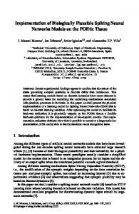
The results shown in Fig 10(a) and Fig 10(b) indicate that the 4-5 Hz of theta band, the 13-14 Hz of alpha band, the 3031 Hz of upper beta band and 34-36 Hz, and 39-40 Hz in lower gamma band are more effective for recognition of negative vs. positive emotions from EEG signal using the MSCE features. Furthermore, the MSCE features at 10-12 Hz upper alpha band and 17-18 Hz, and 27-28 Hz of beta band 37-38 Hz of gamma band are more useful for recognition of arousal level using MSCE features. Since the population of all features is 1000, the red line shown in Fig 10 indicates the P value  0.05 . In addition, a better conclusion can be made when the effective channels at these frequencies are provided as are shown in Table III, and Table IV. Table III. The effective EEG channels for Valence level recognition

Effective frequency (Hz) 4-5 13-14 30-31 34-46 39-40

Effective Channel Channel i Channel j F3 C3, C4 (1/3 C3) C3, C4 (1/5 C3) F3 P4 T7 T7 P4,T8 T8 T7

The results presented in Table III indicate that perception of valence level of emotional stimuli are more detectable based on functional connectivity between left frontal region (F3) and central regions (C3, C4) of the brain at lower EEG frequencies (theta and alpha bands) or based on functional connectivity between parietal (P4) and temporal regions (T7, T8) at upper EEG frequencies (beta and gamma bands). Table IV. The effective EEG channels for Arousal level recognition

Effective frequency (Hz) 10-12 17-18 27-28 37-38

Effective Channel Channel i Channel j C4 F4, P4 F3 T8 P4 C4 T8 F3

Fig 11. The most effective connectivity features for valence (left) and arousal (right) level discrimination

It can be concluded from the results that brain has different policies (functional connectivity patterns) for recognition of valence and arousal level of the emotion. This phenomenon would be very useful in applications such as the improvement of the brain plasticity [69, 70] or the investigation of brain aging using various types of stimuli. There are evidences for a global posterior-anterior shift in aging [71]. However, it should be noted that these results are based on 8 EEG channels and using audio-visual stimulus. Furthermore, obtaining the network parameters using other adaptive methods such as [72] should be considered instead of using GA algorithm for optimizing them. However, as is shown in Table II, the mutual information doesn’t lead to a good network performance, therefore, looking for a better adaptive method is suggested in future works. V. Conclusion This paper presents a biological plausible feed-forward neural network discriminating emotion from EEG based on valence and arousal levels. The EEG data from the perception of emotional stimuli in healthy participants are collected. The top-down approach is formulated and bottom-up approach is bypassed using SAM answers. Subsequently, the performance of the proposed neural network for discriminating emotions is evaluated using the EEG data and SAM responses. The results show that there are patterns of brain regions connectivity in the perception of individual emotional stimuli. These patterns are detectable by estimating the connectivity between different brain regions from the EEG data. However, these patterns vary in different subjects but common patterns can be selected at

10

Manuscript ID TNN-2011-P-3605 specific frequencies. Nevertheless, the feed-forward architecture is presented by considering a constant level of attention, mood and mental health for all subjects. Therefore, further assessment for understanding the impact of attention level, moods and mental disorders on perception of emotional stimuli should be done. In addition, improvement of the network for multi-class valence/arousal problem is proposed for the future works.

[17]

[18] [19] [20]

[21]

Acknowledgment The authors would like to thank Mr. Michel Heijnen and Mrs. Sau Wei Tan for their support in the data collection of the experiment and Drs. Björn Crüts for his valuable advice on designing the experiment.

[22]

References

[24]

[1] [2] [3]

[4]

[5]

[6]

[7] [8]

[9]

[10]

[11]

[12]

[13]

[14]

[15]

[16]

R. W. Picard, Affective computing, Cambridge, Mass.: MIT Press, 2000. P. Ekman, “Facial expression and emotion,” American Psychologist, vol. 48, no. 4, pp. 384-392, 1993. T. Baumgartner, M. Esslen, and L. Jäncke, “From emotion perception to emotion experience: Emotions evoked by pictures and classical music,” International Journal of Psychophysiology, vol. 60, no. 1, pp. 34-43, 2006. M. L. Phillips, “Understanding the neurobiology of emotion perception: implications for psychiatry ” British Journal of Psychiatry vol. 182, pp. 190-192, 2003 R. Adolphs, H. Damasio, D. Tranel et al., “Cortical systems for the recognition of emotion in facial expressions,” The Journal of Neuroscience, vol. 16, no. 23, pp. 7678-7687, December 1, 1996. J. G. Taylor, K. Scherer, and R. Cowie, “Emotion and brain: Understanding emotions and modelling their recognition,” Neural Network, vol. 18, no. 4, pp. 313-316, 2005. K. Oatley, and P. N. Johnson-Laird, “Towards a cognitive theory of emotions,” Cognition & Emotion, vol. 1, pp. 29-50, 1987. R. Khosrowabadi, H. C. Quek, A. Wahab et al., "EEG-based emotion recognition using self-organizing map for boundary detection." pp. 4242-45. J. Lin, M. Spraragen, J. Blythe et al., “EmoCog : Computational integration of emotion and cognitive architecture,” in TwentyFourth International Florida Artificial Intelligence Research Society Conference, Florida, USA, 2011. R. Cowie, and R. R. Cornelius, “Describing the emotional states that are expressed in speech,” Speech Communication, vol. 40, no. 1-2, pp. 5-32, 2003. R. Khosrowabadi, A. Wahab, K. K. Ang et al., "Affective computation on EEG correlates of emotion from musical and vocal stimuli." pp. 1168-72. J. Kim, and E. Andre, “Emotion recognition based on physiological changes in music listening,” IEEE Transactions on Pattern Analysis and Machine Intelligence, vol. 30, no. 12, pp. 2067 - 2083, 2008. R. W. Picard, E. Vyzas, and J. Healey, “Toward machine emotional intelligence: Analysis of affective physiological state,” IEEE Transactions on Pattern Analysis and Machine Intelligence, vol. 23, no. 10, pp. 1175-1191, 2001. M. Pantic, and L. J. M. Rothkrantz, “Automatic analysis of facial expressions: the state of the art,” IEEE Transactions on Pattern Analysis and Machine Intelligence, vol. 22, no. 12, pp. 14241445, 2000. J. C. Borod, and N. K. Madigan, "Neuropsychology of emotion and emotional disorders: An overview and research directions," Neuropsychology of Emotion, J. C. Borod, ed., pp. 3-28, New York: Oxford University Press, 2000. S. G. Costafreda, M. J. Brammer, A. S. David et al., “Predictors of amygdala activation during the processing of emotional stimuli: A meta-analysis of 385 PET and fMRI studies,” Brain Research Reviews, vol. 58, no. 1, pp. 57-70, 2008.

[23]

[25]

[26]

[27] [28] [29]

[30]

[31] [32]

[33] [34] [35]

[36]

[37] [38]

[39] [40]

[41]

[42]

T. Canli, Z. Zhao, J. E. Desmond et al., “An fMRI study of personality influences on brain reactivity to emotional stimuli,” Behavioral Neuroscience, vol. 115, no. 1, pp. 33-42, 2001. R. Adolphs, “Neural systems for recognizing emotion,” Current Opinion in Neurobiology, vol. 12, no. 2, pp. 169-177, 2002. R. H. Hall, "Explicit and implicit memory," 1998]. H. Kober, L. F. Barrett, J. Joseph et al., “Functional grouping and cortical-subcortical interactions in emotion: A meta-analysis of neuroimaging studies,” NeuroImage, vol. 42, no. 2, pp. 998-1031, 2008. M. D. Lewis, and R. M. Todd, “The self-regulating brain: Corticalsubcortical feedback and the development of intelligent action,” Cognitive Development, vol. 22, no. 4, pp. 406-430, 2007. G. C. De Angelis, I. Ohzawa, and R. D. Freeman, “Receptive-field dynamics in the central visual pathways,” Trends in Neurosciences, vol. 18, no. 10, pp. 451-458, 1995. E. D. Jarvis, O. Gunturkun, L. Bruce et al., “Avian brains and a new understanding of vertebrate brain evolution,” Nat Rev Neurosci, vol. 6, no. 2, pp. 151-159, 2005. E. R. Kandel, In search of memory: the emergence of a new science of mind: W.W. Norton & Co., 2007. K. N. Ochsner, and J. J. Gross, "The neural architecture of emotion regulation," Handbook of Emotion Regulation, J. J. Gross, ed., pp. 87-109, New York: The Guilford Press, 2009. T. Brosch, G. Pourtois, and D. Sander, “The perception and categorisation of emotional stimuli: A review,” Cognition & Emotion, vol. 24, no. 3, pp. 377-400, 2010. K. R. Scherer, A. Schorr, and T. Johnstone, Appraisal processes in emotion, USA: Oxford university press, 2001. E. T. Rolls, The brain and emotion: Oxford University Press, 1999. P. J. Lang, M. M. Bradley, and B. N. Cuthbert, International affective picture system (IAPS): Affective ratings of pictures and instruction manual, Technical Report A-6, University of Florida, Gainesville, FL, 2005. M. Esslen, R. D. Pascual-Marqui, D. Hell et al., “Brain areas and time course of emotional processing,” NeuroImage, vol. 21, no. 4, pp. 1189-1203, 2004. J. Kim, Philosophy of mind, 3 ed., p.^pp. 384: Westview Press, 2010. J. Musch, and K. C. Klauer, The psychology of evaluation: affective processes in cognition and emotion: Lawrence Erlbaum Associates, 2003. O. Sporns, “Brain connectivity,” Scholarpedia, vol. 2, no. 10, pp. 4695, 2007. S. M. Kay, Modern spectral estimation: Theory and application, Englewood Cliffs, NJ.: Prentice Hall, 1988. G. Carter, C. Knapp, and A. Nuttall, “Estimation of the magnitude-squared coherence function via overlapped fast Fourier transform processing,” Audio and Electroacoustics, IEEE Transactions on, vol. 21, no. 4, pp. 337-344, 1973. R. Zass, and A. Shashua, "Nonnegative Sparse PCA," Advances in Neural Information Processing Systems 19, B. Schölkopf, J. Platt and T. Hoffman, eds., Cambridge, MA: MIT Press, 2007. A. J. Flugge, S. Olhede, and M. Fitzgerald, “Non-negative PCA for EEG-Data Analysis,” Interpreting, vol. 101, pp. 776-780, 2009. S. Chen, C. F. N. Cowan, and P. M. Grant, “Orthogonal least squares learning algorithm for radial basis function networks,” IEEE Transactions on Neural Networks, vol. 2, no. 2, pp. 302309, 1991. H. Demuth, and M. Beale, "Neural network toolbox for use with Matlab," Mathworks, 1998. J. Park, and I. W. Sandberg, “Universal approximation using radial-basis-function networks,” Neural Computation, vol. 3, no. 2, pp. 246-257, 1991. G.-B. Huang, Q.-Y. Zhu, and C.-K. Siew, “Extreme learning machine: Theory and applications,” Neurocomputing, vol. 70, no. 1-3, pp. 489-501, 2006. P. D. Wasserman, Advanced methods in neural computing: John Wiley &Sons, Inc., 1993.

11

Manuscript ID TNN-2011-P-3605 [43]

[44] [45]

[46]

[47]

[48] [49]

[50] [51]

[52] [53]

[54]

[55]

[56] [57]

[58]

[59]

[60]

[61]

[62]

[63]

[64]

[65] [66]

T. Cover, and P. Hart, “Nearest neighbor pattern classification,” IEEE Transactions on Information Theory, vol. 13, no. 1, pp. 2127, 1967. W. J. Krzanowski, Principles of multivariate analysis:A user's perspective, USA: Oxford University Press, 2000. N. Cristianini, and J. Shawe-Taylor, An Introduction to support vector machines and other kernel-based learning methods: Cambridge University Press, 2000. P. C. Petrantonakis, and L. J. Hadjileontiadis, “Emotion recognition from EEG using higher order crossings,” IEEE Transactions on Information Technology in Biomedicine, vol. 14, no. 2, pp. 186-197, 2010. M. Murugappan, N. Ramachandran, and Y. Sazali, “Classification of human emotion from EEG using discrete wavelet transform ” Journal of Biomedical Science and Engineering, vol. 3, no. 4, pp. 390-396, April 2010, 2010. A. Ortony, and T. J. Turner, “What's basic about basic emotions?,” Psychological Review, vol. 97, no. 3, pp. 315-331, 1990. P. Ekman, "Basic emotions," Handbook of Cognition and Emotion, T. Dagleish and M. Power, eds., pp. 45-60, Sussex, U.K.: John Wiley & Sons Ltd., 1999. C. E. Izard, Human emotions, New York: Plenum Press, 1977. R. Plutchik, "A general psychoevolutionary theory of emotion," Emotion: Theory, research, and experience, R. Plutchik and H. Kellerman, eds., pp. 3-33, New York: Academic Press, 1980. J. A. Russell, “A circumplex model of affect,” Journal of personality and social psychology vol. 39, pp. 1161 - 1178, 1980. P. J. Lang, "Behavioral treatment and bio-behavioral assessment: Computer applications," Technology in Mental Health Care Delivery Systems, J. Sidowski, J. Johnson and T. Williams, eds., pp. 119-137, Norwood, NJ: Ablex Pub. Corp., 1980. M. M. Bradley, and P. J. Lang, The international affective digitized sounds (2nd Edition; IADS-2): Affective ratings of sounds and instruction manual, Technical report B-3, University of Florida, Gainesville, Fl, 2007. S. Vieillard, I. Peretz, N. Gosselin et al., “Happy, sad, scary and peaceful musical excerpts for research on emotions,” Cognition & Emotion, vol. 22, no. 4, pp. 720 - 752, 2008. J. J. Gross, and R. W. Levenson, “Emotion elicitation using films,” Cognition & Emotion, vol. 9, no. 1, pp. 87-108, 1995. V. V. Kulish, A. I. Sourin, and O. Sourina, “Fractal spectra and visualization of the brain activity evoked by olfactory stimuli,” in the 9th Asian Symposium on Visualization, Hong Kong, 2007. G. Chanel, J. J. M. Kierkels, M. Soleymani et al., “Short-term emotion assessment in a recall paradigm,” Int. J. Hum.-Comput. Stud., vol. 67, no. 8, pp. 607-627, 2009. R. C. Oldfield, “The assessment and analysis of handedness: The Edinburgh inventory,” Neuropsychologia, vol. 9, no. 1, pp. 97113, 1971. P. Fusar-Poli, A. Placentino, F. Carletti et al., “Laterality effect on emotional faces processing: ALE meta-analysis of evidence,” Neuroscience Letters, vol. 452, no. 3, pp. 262-267, 2009. R. W. Thatcher, C. J. Biver, and D. North, "EEG coherence and phase delays: Comparisons between single reference, average reference and current source density," Neurology in Version 1, University of South Florida College of Medicine, 2004. B. Hjorth, “EEG analysis based on time domain properties,” Electroencephalography and clinical neurophysiology, vol. 29, no. 3, pp. 306-310, 1970. R. Khosrowabadi, C. Quek, K. K. Ang et al., “A brain-computer interface for classifying EEG correlates of chronic mental stress,” in IEEE International Joint Conference on Neural Networks, San Jose, California,USA, 2011, pp. 757-762. D. Whitley, "Genetic algorithms and neural networks " Genetic Algorithms in Engineering and Computer Science., Winter, Periaux, Galan et al., eds., pp. 203-216: John Wiley & Sons Ltd, 1995. J. Beran, Statistics for long-memory processes, Florida, USA: Chapman & Hall, 1994. P. Flandrin, “Wavelet analysis and synthesis of fractional Brownian motion,” IEEE Transactions on Information Theory, vol. 38, no. 2, pp. 910-917, 1992.

[67]

[68]

[69]

[70]

[71]

[72]

J. Istas, and G. Lang, “Quadratic variations and estimation of the local Hölder index of a Gaussian process,” Annales de l'Institut Henri Poincare (B) Probability and Statistics, vol. 33, no. 4, pp. 407-436, 1997. P. Abry, P. Flandrin, M. S. Taqqu et al., "Self-similarity and longrange dependence through the wavelet lens," Theory and Applications of Long-Range Dependence, P. Doukhan, G. Oppenheim and M. S. Taqqu, eds., pp. 527-556, Boston, MA: Birkhauser, 2000. J. Doyon, and H. Benali, “Reorganization and plasticity in the adult brain during learning of motor skills,” Current Opinion in Neurobiology, vol. 15, no. 2, pp. 161-167, 2005. H. W. Mahncke, A. Bronstone, and M. M. Merzenich, "Brain plasticity and functional losses in the aged: scientific bases for a novel intervention," Progress in Brain Research, R. M. Aage, ed., pp. 81-109: Elsevier, 2006. S. W. Davis, N. A. Dennis, S. M. Daselaar et al., “Qué PASA? The posterior–anterior shift in aging,” Cerebral Cortex, vol. 18, no. 5, pp. 1201-1209, May 1, 2008, 2008. P. C. Petrantonakis, and L. J. Hadjileontiadis, "Adaptive extraction of emotion-related EEG segments using multidimensional directed information in time-frequency domain." pp. 1-4.