Combined finite volume and finite element method for convection

Journal of

Journal of Mechanical Science and Technology 23 (2009) 790~801

Mechanical Science and Technology www.springerlink.com/content/1738-494x

DOI 10.1007/s12206-008-1204-0

Combined finite volume and finite element method for convection-diffusion-reaction equation† Sutthisak Phongthanapanich1 and Pramote Dechaumphai2,* 1

Department of Mechanical Engineering Technology, College of Industrial Technology, King Mongkut’s University of Technology North Bangkok, Bangkok 10800, Thailand 2 Mechanical Engineering Department, Chulalongkorn University, Bangkok 10330, Thailand (Manuscript Received May 15, 2008; Revised November 25, 2008; Accepted December 11, 2008) --------------------------------------------------------------------------------------------------------------------------------------------------------------------------------------------------------------------------------------------------------

Abstract A combined finite volume and finite element method is presented for solving the unsteady scalar convectiondiffusion-reaction equation in two dimensions. The finite volume method is used to discretize the convection-diffusionreaction equation. The higher-order reconstruction of unknown quantities at the cell faces is determined by Taylor's series expansion. To arrive at an explicit scheme, the temporal derivative term is estimated by employing the idea of local expansion of unknown along the characteristics. The concept of the finite element technique is applied to determine the gradient quantities at the cell faces. Robustness and accuracy of the method are evaluated by using available analytical and numerical solutions of the two-dimensional pure-convection, convection-diffusion and convectiondiffusion-reaction problems. Numerical test cases have shown that the method does not require any artificial diffusion to improve the solution stability. Keywords: Convection-diffusion-reaction equation; Explicit method; Finite volume method; Finite element method --------------------------------------------------------------------------------------------------------------------------------------------------------------------------------------------------------------------------------------------------------

1. Introduction Mathematical models of physical, chemical, biological, and environmental phenomena are governed by various forms of partial differential equations. The partial differential equations describing the transport phenomena in fluid dynamics [1-4] are particularly difficult due to the convection terms. Such equations represent the hyperbolic conservation law for which their solutions always contain discontinuity and high gradient; thus accurate numerical solutions are very difficult to obtain. Special treatment must be applied to suppress spurious oscillations of the computed solutions for both the pure convection and convection-dominated problems [5-8]. At present, better †This paper was recommended for publication in revised form by Associate Editor Dongshin Shin * Corresponding author. Tel.: +66 2 218 6621, Fax.: +66 2 218 6621 E-mail address: [email protected] © KSME & Springer 2009

ways to approximate the convection term are still needed, and thus development of accurate numerical modeling for the convection-diffusion equations remains a challenging task in computational fluid dynamics [1-11]. The explicit method is popular because it is simple and parallelizable. However, the method is limited by the CFL stability criterion and thus a small time step is required to stabilize the computational procedure. On the other hand, the implicit method is unconditionally stable, but larger time step may not be used because the solution accuracy degrades as it proceeds in time. The inversion of the coefficient matrix is another weakness of the method because it is a timeconsuming process. To simulate large scale industrial applications, the available memory is a crucial aspect that must be considered. The explicit method is thus preferred in the development of new algorithms. The objective of this work is to develop an explicit

791

S. Phongthanapanich and P. Dechaumphai / Journal of Mechanical Science and Technology 23 (2009) 790~801

finite volume/finite element method that can provide stabilized numerical solutions for unsteady scalar convection-diffusion-reaction problems. The combination of the conventional finite element and finite volume methods for analyzing fluid flow problems is of interest to many researchers [12-14]. In this paper, an explicit finite volume method is employed to derive the discretized equations for the spatial domain. The higher-order solution is approximated by extending the idea of references [15-17] to determine the numerical flux along the cell face at the half time step by f = f (φijn+1/ 2 ) . To formulate the numerical scheme in an explicit form, the temporal term is estimated by adopting the idea of the local expansion of unknowns along the characteristics [18-19]. Robustness and efficiency of the proposed method are examined by analyzing the pure convection, convectiondominated diffusion, and convection-diffusion-reaction problems. The presentation of the paper starts from the explanation of the theoretical formulation in Section 2. The performance of proposed method is then evaluated in Section 3 by using four examples: (1) the square pulse flow in a square domain, (2) the rotation of two Gaussian pulses, (3) the triangular wave inflow convection, and (4) the skewed convection problem with influence of reaction.

2. Finite volume element formulation The governing partial differential equation for the unsteady scalar convection-diffusion-reaction problem can be written in the form as

∂φ + ∇ ⋅ (vφ − ε∇φ ) + κφ = q ∂t

∫ ∫ Ωi

t

n

1 Ωi

φin =

∫ φ ( x,t )dx n

Ωi

1 Ωi

φin +1 =

∫ φ ( x, t

⎛ ∂φ ⎞ + ∇ ⋅ (vφ − ε∇φ ) + κφ − q ⎟dtdx = 0 (2) ⎜ ⎝ ∂t ⎠

In the conventional finite volume method, the ap-

n +1

Ωi

and

)dx

(3)

where Ωi is the measure of Ω i . Next, the temporal integration and the divergence theorem are applied to the first and the second term of Eq. (2), respectively. With the use of Eq. (3), Eq. (4) is obtained:

φin +1 = φin − +

∆t Ωi

⎡ ⎢ ⎢⎣

∫ ∫ Ωi

t n+1

∫ ∫ n (υ ) ⋅ (v(υ )φ (υ, t ) − ε∇φ (υ, t ))dυdt i ∂Ω i

tn

t n+1

t

κφ ( x, t )dtdx − n

∫ ∫ Ωi

t

⎤ q ( x , t )dtdx ⎥ ⎥⎦

t n +1 n

(4)

For an arbitrary control volume Ωi , the flux integral over ∂Ωi appearing on the right-hand side of Eq. (4) could be approximated by the summation of the fluxes passing through all adjacent cell faces. Hence, by applying the midpoint quadrature integration rule for both the temporal and spatial domain terms, the flux integral over ∂Ωi may be approximated by t n+1

∫ ∫ n (υ ) ⋅ (v(υ )φ (υ, t ) − ε∇φ (υ ,t ))dυdt i ∂Ω i

tn

∑ Γ n ⋅ (v φ (t NF

(1)

where φ is the unknown scalar quantity, v = v (x ) is the given convection velocity field, ε ≥ 0 is the diffusion coefficient, κ is the reaction coefficient, q = q( x, t ) is the prescribed source term, and t ∈ (0, T ) with T > 0 . The initial condition is defined for x ∈ Ω and Ω ⊂ R 2 by φ ( x,0) = φ0 ( x ) . Equation (1) is then integrated over an arbitrary control volume Ω i and in the time interval (t n , t n +1 ) to obtain t n+1

proximation to the cell average of φ over Ω i at time t n and t n +1 is represented by

=

ij

ij

ij ij

n +1 / 2

) − ε∇φij (t n +1 / 2 )

)

(5)

j =1

where NF is the number of the surrounding control volumes, and Γij is the segment of boundary ∂Ωi between the two adjacent control volumes Ω i and Ω j , which is defined by ∂Ωi = ∪ NF and j =1 Γij Γij = ∂Ωi ∩ ∂Ω j . It should be noted that ∇φij (t n +1 / 2 ) is approximated by ∇φij (t n ) throughout this paper for simplicity. The integrations of the reaction and source terms can be also approximated by

∫ ∫ Ωi

∫ ∫ Ωi

t n+1

tn

t n +1 tn

κφ ( x, t )dtdx = Ωi κφin +1 / 2

(6)

q( x, t )dtdx = Ωi qi (t n+1/ 2 )

(7)

792


By substituting Eqs. (5)-(7) into Eq. (4), an explicit finite volume scheme for solving Eq. (1) can be written in the form

φin+1 = φin −

∆t Ωi

NF

∑Γ j =1

ij

(

nij ⋅ vijφijn+1/ 2 − ε∇φijn

−∆t (κφin+1/ 2 − qin+1/ 2 )

) (8)

where the quantities at time t n+1/ 2 are φijn+1/ 2 = φij (t n+1/ 2 ) , φijn = φij (t n ) , φin+1/ 2 = φi (t n+1/ 2 ) , and qin+1/ 2 = qi (t n+1/ 2 ) . The gradient term, ∇φijn , is determined by the weighted residuals method, which is commonly used in the finite element technique [20]. First, this ∇φijn is assumed to distribute linearly over Ωi in the form NP

∇φ = ∑ N j ( x )∇φ n i

j =1

n j

(9)

where NP is the number of control volume vertices, and N j ( x ) denotes the linear interpolation functions for the adjacent control volumes. By applying the weighted residuals method and Gauss’s theorem to Eq. (9), the gradient quantities at the grid point are obtained as ∇φ jn,i = M −1

−∫

(∫

∂N j (υ ) Ωi

∂x

∂Ωi

ni (υ ) N j (υ )φin dυ

⎞

φin dx ⎟ ⎠

(10)

where M is the consistent mass matrix [20], and ∇φ nj ,i are the contributions of the gradient quantities in the control volume Ωi to the gradient quantities at the grid point j. The nodal gradient approximation in Eq. (10) is similar to that used in the control volume finite element method suggested by Swaminathan et al. [21] for discretizing the diffusion flux. Equation (10) is presented in a simple form herein so that it can be applied conveniently to the unstructured grid. To compute the total gradient quantities at node j, Eq. (10) is applied to all control volumes I surrounding the grid point j such that I

∇φ jn = ∑ ∇φ jn,i

puted by applying the midpoint quadrature integration rule along the edge connected to grid point i and j. Finally, the scalar quantity at the half time step t n +1 / 2 , φijn +1 / 2 , is approximated by applying the Taylor's series expansion in both space and time [15-17]. Similarly, the scalar quantity, φin +1 / 2 , is approximated by applying the Taylor's series expansion in time. To obtain the explicit numerical scheme, the temporal derivative term is determined by utilizing the idea of local expansion of unknown along the characteristics [18]. By assuming that the velocity points in the direction from Ωi to Ω j , the values of φijn +1 / 2 and φin +1 / 2 can be written as

φijn+1/ 2 = φin + ( xij − xi ) ⋅ ∇φin − φin+1/ 2 = φin −

∆t ( vi ⋅ ∇φin ) 2

∆t ( vi ⋅ ∇φin ) 2

(12) (13)

For the opposite direction of velocity, the values of φijn +1 / 2 and φin +1 / 2 could be computed from Eqs. (12) and (13), respectively, but using the values from the neighboring triangles according to the upwinding direction.

3. Accuracy and stability analysis For simplicity, the order of accuracy and the stability of the explicit numerical scheme [22] given by Eq. (8) are analyzed on a uniform one-dimensional grid cell, Ωi = ∆x , and at a constant velocity of a > 0. The homogeneous unsteady convection-diffusion equation for the ith cell, Ωi ∈ ( xi −1 / 2 , xi +1 / 2 ) , may be written in a semi-discrete form as

φin+1 = φin − −ε (

∂φ ∂x

∆t ⎡ n+1/ 2 n+1/ 2 ⎢ a(φi+1/ 2 − φi−1/ 2 ) ∆x ⎣

n

− i +1/ 2

∂φ ∂x

⎤ )⎥ i −1/ 2 ⎥ ⎦ n

(14)

By using the linear interpolation function as described above together with Eq. (12), the cell-centered finite volume-based finite element equation for Eq. (14) is

φin+1 = φin − R(φin − φin−1 ) (11)

i =1

The gradient quantities at Γij , ∇φijn , are then com-

R (1 − R ) n (φi − 2φin−1 + φin−2 ) 2 + r (φin+1 − 2φin + φin−1 ) −

(15)

793


∆t ∆t and r = ε 2 . Eq. (15) represents ∆x ∆x the second-order one-sided upwind-space approximation and the centered-space approximation for the convective and diffusive terms, respectively. Hence, the order of accuracy for the numerical scheme is O(∆t 2 , ∆x 2 ) . To investigate the stability, the discrete Fourier transform is applied term by term to Eq. (15). The amplification factor, G, corresponding to Eq. (15) is

1

where R = a

3 R2 R+ + R(2 − R)cos ξ 2 2 R ( R − 1) ξ + cos 2ξ ) − 4r sin 2 2 2 R( R − 1) − I ( R(2 − R )sin ξ + sin 2ξ ) 2

G = (1 −

(16)

Due to the complexity of Eq. (16) above, it is solved numerically by varying parameters with small increments to ensure the stability of the numerical scheme on an arbitrary cell. For stability, R should satisfy the CFL stability criterion. Herein, the time-step within each cell is determined from 2 ⎛ Γic ⎞⎟ Ωi ⎜ , ∆t = C min⎜ ⎟ i ⎜ max j =1, 2,3 v n, ij 2ε ⎟ ⎠ ⎝

(17)

where vn,ij is the scaled normal velocity at Γij , Γic is the characteristic length of cell i, and 0 < C ≤1.

4. Numerical examples To evaluate the robustness and accuracy of the combined finite volume and finite element method, examples of pure-convection, convection-diffusion and convection-diffusion-reaction problems are examined. All examples presented in this section were tested by using square grids. These examples are: (1) square pulse flow in a square domain, (2) rotation of two Gaussian pulses, (3) triangle wave inflow convection, and (4) skewed convection problem with influence of reaction. 4.1 Square pulse flow in a square domain

The first example is adopted from the paper presented by Waterson and Deconinck [23]. It is a con-

y

0.75

0.5

0.25

0

0

(a) Grid S1

0.25

0.5

x

0.75

1

(b) Exact

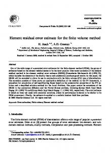
Fig. 1. Typical uniform grid S1 and exact solution of problem 4.1.

vection problem with the unknown of a scalar quantity from non-uniform flow field in a unit square domain, Ω = (0,1) × (0,1) . The initial condition φ0 ( x ) is set to be zero and the inflow boundary condition along the boundary y = 0 is given by

⎧1 ⎩0

φ0 ( x ) = ⎨

0.4 ≤ x ≤ 0.6 otherwise

(18)

The steady-state velocity field is specified as

u ( x ) = x and v(x ) = 1 − y

(19)

Because of the sudden change of the flow profile at the outflow boundary x = 1 , spurious oscillations of the computed solution may occur along that boundary. To eliminate these artifacts of the computed solution along such outflow boundary, the Barth and Jespersen limiter function [24] is imposed. The uniform grids S1 to S4 consisting of 32 × 32 ( ∆x = ∆y = 1 32 ), 64 × 64, 128 × 128, and 256 × 256 cells, respectively, are used in this example. Figs. 1(a)-(b) show a typical grid S1 and the exact steady-state solution. Figs. 2(a)-(d) show the numerical solutions of the four uniform grids S1 to S4, respectively. Fig. 3 shows the computed profiles along the outflow boundary x = 1 obtained from grids S1 to S4 as compared to the exact solution. The computed profiles obtained from these grids approach the exact solution as the grid is refined. Figure 4 shows the plot of L1 -norm errors of the solutions versus grid sizes. It is noted that the experimental order of convergence (EOC) of the L1 -norm error for this problem is less than one due to the effect of the limiter function. The minimum and maximum values obtained from the grid S4 are -0.0065 and 1.003, respectively. By comparing these computed solutions with the exact minimum and maximum values of 0 and 1, respec-

794


tively, the proposed method can provide a solution that converges to the exact solution as the grid is refined. 4.2 Rotation of two gaussian pulses

(a) Grid S1

(b) Grid S2

To evaluate the performance of the proposed method for solving pure convection and convectiondominated diffusion problems, the example of the two Gaussian pulses scalar field rotating around the domain Ω = (−0.5,−0.5) × (0.5,0.5) is selected. This problem is adopted from the example presented by Wang et al. [25] for which the initial condition is given by

φ0 ( x ) = max( f ( xc1 ), f ( xc2 )) (c) Grid S3

(20)

(d) Grid S4

Fig. 2. Numerical solutions of grids S1 to S4 of problem 4.1.

and

⎛ ( x − xc ) 2 + ( y − y c ) 2 i i f ( x ci ) = exp⎜ − 2 ⎜ 2σ ⎝

⎞ ⎟ ⎟ ⎠

(21)

where xc1 and xc2 are the center coordinates of the Gaussian pulses which are (−0.25,0) and (0.25,0) , respectively. The standard deviation is given by σ = 0.0447 . The rotating velocity field with the angular velocity of 4 rad/s is

u ( x ) = −4 y and v( x ) = 4 x

Fig. 3. Comparison of exact and numerical solutions of grids S1 to S4 of problem 4.1.

Fig. 4. Experimental order of convergence of the L1 -norm error of problem 4.1.

(22)

The final time is selected as π 2 , which is the time period required for one turn rotation. To determine the EOC value of the proposed method, a refined grid S5 (512 × 512) is included in addition for this example. The first test case is a pure convection problem. The contour and the 3D contour plots of the exact and numerical solutions from the three uniform grids S1, S2, and S3, are presented in Figs. 5(a)-(d), respectively. The comparison of the exact and numerical solutions (S1 to S5) along the line y = 0 passing through the two apexes of Gaussian pulses is shown in Fig. 6. It is noted that the numerical solution obtained from the refined grid S5 coincides with the exact solution. These figures show that, by comparing with the exact minimum of 0 and maximum of 1, the proposed method provides a solution that converges to the exact solution as the grid is refined. To determine the EOC value of the method, Fig. 7 plots the

795

S. Phongthanapanich and P. Dechaumphai / Journal of Mechanical Science and Technology 23 (2009) 790~801 1

0.8

Exact S1 S2 S3 S4 S5

0.6

scalar

L1 -error norms versus grid sizes for the sequence of grid S2 to S5. This figure shows that the EOC value for this first test case is around two. Results obtained from the proposed method (FVEM), the conventional finite volume method (FVM) with second-order TVD Runge-Kutta time stepping [15], and the characteristic Galerkin finite element method (CFEM) [19,20] are compared in Fig. 8. Figure 9 compares the distributions obtained from three methods using grid S3 with the exact solution along the line y = 0 . The figure shows that the FVM gives a smeared distribution of the solution. The solution obtained from

0.4

0.2

0 -0.5

0

0.5

x

Fig. 6. Comparison of numerical solutions along the line y = 0 of problem 4.2 ( ε = 0 ).

Log(h)

-3 0

-2

-1

-1

(a) Exact -2 2.13

Log(||L1||)

-3

-4

-5

(b) Grid S1

Fig. 7. Experimental order of convergence of the L1 -norm error of problem 4.2 ( ε = 0 ).

(c) Grid S2 (a) FVEM

(b) FVM

(d) Grid S3

(c) CFEM

Fig. 5. Comparison of exact and numerical solutions of grids S1, S2, and S3 of problem 4.2 ( ε = 0 ).

Fig. 8. Comparison of three numerical schemes on grid S3 of problem 4.2 ( ε = 0 ).

796

S. Phongthanapanich and P. Dechaumphai / Journal of Mechanical Science and Technology 23 (2009) 790~801 1

1

0.8

Exact FVEM FVM CFEM

0.8

Exact S1 S2 S3 S4 S5

scalar

0.6

scalar

0.6 0.4

0.4 0.2

0.2 0 -0.5

0

x

0.5

Fig. 9. Comparison of numerical solutions along the line y = 0 on grid S3 of problem 4.2 ( ε = 0 ).

0 -0.5

0

0.5

x

Fig. 11. Comparison of numerical solutions along the line y = 0 of problem 4.2 ( ε = 10 −4 ). Log(h)

-3 0

-2

-1

-1

-2

(a) Exact

1.95

Log(||L1||)

-3

-4

-5

(b) Grid S1

(c) Grid S2

(d) Grid S3 Fig. 10. Comparison of exact and numerical solutions of grids S1, S2, and S3 of problem 4.2 ( ε = 10 −4 ).

Fig. 12. Experimental order of convergence of the L1 -norm error of problem 4.2 ( ε = 10 −4 ).

CFEM is comparable with FVEM but is less accurate. In addition, the CFEM yields a solution with small oscillation behind the two Gaussian pulse profiles. The second test case is a convection-dominated diffusion problem with a diffusion coefficient of ε = 10−4 . The contour and the 3D contour plots of the exact and numerical solutions are presented in Figs. 10(a)-(d). The comparison of the exact and numerical solutions along the line y = 0 is also shown in Fig. 11. These figures again show that, by comparing with the exact minimum of 0 and maximum of 0.8642, the proposed method again provides a solution that converges to the exact solution as the grid is refined. Fig. 12 plots the L1 -error norms versus grid sizes for the sequence of grids S2 to S5, and the EOC value for this second test is also around two. A comparison of the results obtained from the three methods for this case is presented in Fig. 13. Fig. 14


(a) FVEM

797

(b) FVM

(a) Exact

(b) Grid S1

(c) CFEM Fig. 13. Comparison of three numerical schemes on grid S3 of problem 4.2 ( ε = 10 −4 ). 1

0.8

Exact FVEM FVM CFEM

0.6

scalar

(c) Grid S2

(d) Grid S3

Fig. 15. Comparison of exact and numerical solutions of grids S1, S2, and S3 of problem 4.3.

0.4

0.2

0 -0.5

0

0.5

x

Fig. 14. Comparison of numerical solutions along the line y = 0 on grid S3 of problem 4.2 ( ε = 10 −4 ).

compares the solutions obtained from three methods using grid S3 with the exact solution along the line y = 0 . The solution behaviors are similar to the previous case, i.e., the FVM yields a smeared solution while the solution obtained from the CFEM is less accurate than that from the FVEM. It is noted that the CFEM still yields a solution with small oscillation behind the two Gaussian pulse profiles. 4.3 Triangular wave inflow convection

The third example is the triangular wave inflow convection problem on the domain Ω = (0,0) × (1,1) . The initial condition φ0 ( x ) is set to be zero and the boundary condition at x = 0 is given by ⎧100( y − 0.25) ⎪ φ0 ( x = 0, y ) = ⎨100(0.75 − y ) ⎪ 0 ⎩

0.25 ≤ y ≤ 0.5 0.5 < y ≤ 0.75 (23) otherwise

where the steady velocity field is given by u ( x ) = 0.05 and v( x ) = 0 . The profile drops suddenly to zero at the outflow boundary according to the condition on the right side of the domain. To reduce the oscillation at the outflow boundary, the Barth and Jespersen limiter function [24] is imposed. The 3D contour plots of the exact and numerical solutions obtained from using the three uniform grids S1, S2, and S3 at time t = 15 are presented in Figs. 15(a)-(d), respectively. The comparison of the exact and numerical solutions (S1 to S3) along the line x = 0.5 passing through the apex of triangular wave is shown in Fig. 16. There is a small dropping of the amount of its height with slight oscillation behind the front profile. However, these figures show that as the grid size becomes smaller, the front profile is sharper and the oscillation is limited to a few cells behind it. The numerical solutions obtained from the three numerical methods using grid S2 are shown in Fig. 17. The numerical solution obtained from FVEM is comparable with the CFEM solution, while the FVM method produces oscillation along the flow direction. Fig. 18 compares the exact and numerical solutions along the line x = 0.5 . The figure shows that the

798


FVEM method provides higher solution accuracy as compared to the FVM and CFEM methods. 4.4 Skew convection problem with influence of reaction

Fig. 16. Comparison of numerical solutions along the line x = 0.5 of problem 4.3.

(a) FVEM

The last example is a convection-diffusion-reaction problem of a skewed convection with an influence of reaction [6]. The skewed convection flow is determined on a square domain Ω = (0,0) × (1,1) , with the velocity field given by u ( x ) = 0.15 and v( x ) = 0.1 . The initial condition φ 0 ( x ) is set to be zero. The boundary conditions are equal to one along the boundaries x = 0 and y = 1 , and zero along the other boundaries. The diffusion coefficient is specified as ε = 10 −4 , and the grid 20 × 20 is used in the computation. For comparing with the results presented in Ref. [6], the reaction coefficient, κ , is gradually increased as 0, 0.01, 0.1, 1, and 10.

(b) FVM

(a) κ = 0

(b) κ = 0.01

(c) CFEM Fig. 17. Comparison of three numerical schemes on grid S2 of problem 4.3.

(c) κ = 0.1

(d) κ = 1

25

20

Exact FVEM FVM CFEM

scalar

15

10

5

0

0

0.5

x

1

Fig. 18. Comparison of numerical solutions along the line x = 0.5 on grid S2 of problem 4.3.

(e) κ = 10 Fig. 19. Numerical solutions at different reaction coefficients on 20 × 20 grid of problem 4.4.


799

5. Conclusion

(a) κ = 0

(b) κ = 0.01

(c) κ = 0.1

(d) κ = 1

This paper presents an explicit formulation of a combined finite volume and finite element method for solving the unsteady scalar convection-diffusionreaction equation on two-dimensional domain. The theoretical formulation of the proposed method was explained in detail. The finite volume method was applied to derive the discretized equations for the spatial domain, and the concept of the finite element technique is implemented to estimate the gradient quantities at the cell faces. Four numerical examples were used to evaluate the robustness and to determine the order of accuracy of the proposed method. These examples showed that the method can provide a converged solution with improved accuracy as the grid is refined. In addition, the method does not need any artificial diffusion to improve the solution stability.

Acknowledgment The authors are pleased to acknowledge the Thailand Research Fund (TRF) for supporting this research work.

References

(e) κ = 10 Fig. 20. Numerical solutions at different reaction coefficients on unstructured grid of problem 4.4.

The Barth and Jespersen limiter function is imposed herein to eliminate the spurious oscillations of the computed solution in the vicinity of a sudden change in the solution profile. The numerical solutions at the five values of reaction coefficients as given above are shown in Figs. 19(a)-(e), respectively. For comparison purposes, this problem is tested again on an unstructured grid consisting of 1,624 grids (20 cells on each boundary). The numerical solutions are shown in Figs. 20(a)-(e), respectively. The spurious oscillations are completely eliminated and the high quality of the solution profiles is still preserved as compared to those presented in Ref. [6]. Because the explicit artificial diffusion term was not needed during the computation, the numerical solution thus does not suffer from excessive diffusion as it proceeds in time.

[1] P. Frolkovic and H. De Schepper, Numerical modelling of convection dominated transport coupled with density driven flow in porous media, Adv. in Water Res. 24 (1) (2000) 63-72. [2] S. Kim and M. C. Kim, Multi-cellular natural convection in the melt during convection-dominated melting, KSME Int. J. 16 (1) (2002) 94-101. [3] E. Bertolazzi and G. Manzinim, Least square-based finite volumes for solving the advection-diffusion of contaminants in porous media, Appl. Numer. Math. 51 (4) (2004) 451-461. [4] C. Man and C. W. Tsai, A higher-order predictorcorrector scheme for two-dimensional advectiondiffusion equation, Int. J. Numer. Meth. Fluids. 56 (4) (2007) 401-418. [5] R. Codina, A discontinuity-capturing crosswind dissipation for the finite element solution of the convection-diffusion equation, Computer Methods in Applied Mechanics and Engineering, 110 (3-4) (1993) 325-342. [6] L. P. Franca and F. Valentin, On an improved unusual stabilized finite element method for the advective–reactive–diffusive equation, Computer Methods in Applied Mechanics and Engineering, 190

800


(13-14) (2000) 1785-1800. [7] T. Knopp, G. Lube and G. Rapin, Stabilized finite element methods with shock capturing for advection–diffusion problems, Comp. Meth. Appl. Mech. Engrg. 191 (27) (2002) 2997-3013. [8] N. Heitmann and S. Peurifoy, Stabilization of the evolutionary convection-diffusion problem: introduction and experiments, Proceedings of the SSHEMA Spring 2007 Conference, (2007). [9] A. Nesliturk and I. Harari, The nearly-optimal Petrov-Galerkin method for convection-diffusion problems, Comp. Meth. Appl. Mech. Engrg. 192 (22) (2003) 2501-2519. [10] A. Smolianski, O. Shipilova and H. Haario, A fast high-resolution algorithm for linear convection problems: Particle transport method, Int. J. Numer. Meth. Eng. 70 (6) (2007) 655-684. [11] H. Gomez, I. Colominas, F. Navarrina and M. Casteleiro, A discontinuous Galerkin method for a hyperbolic model for convection-diffusion problems in CFD, Int. J. Numer. Meth. Eng. 71 (11) (2007) 1342-1364. [12] R. Swaminathan and V. R. Voller, Streamline upwind scheme for control-volume finite elements, part 1. Formulations, Numer. Heat Tr. Part B. 22 (1) (1992) 95-107. [13] C. Gallo and G. Manzini, Finite volume/mixed finite element analysis of pollutant transport and bioremediation in heterogeneous saturated aquifers, Int. J. Numer. Meth. Fluids. 42 (1) (2003) 1-21. [14] M. S. Chandio, K. S. Sujatha and M. F. Webster, Consistent hybrid finite volume/element formulations: model and complex viscoelastic flows, Int. J. Numer. Meth. Fluids. 45 (9) (2004) 945-971. [15] S. Phongthanapanich and P. Dechaumphai, Twodimensional adaptive mesh generation algorithm and its application with higher-order compressible flow solver, KSME Int. J. 18 (12) (2004) 2190-2203.

[16] M. Ben-Artzi and J. Falcovitz, A second-order Godunov-type scheme for compressible fluid dynamics, J. Comput. Phys. 55 (1) (1984) 1-32. [17] S. J. Billett and E. F. Toro, On WAF-type schemes for multidimensional hyperbolic conservation laws, J. Comput. Phys. 130 (1) (1997) 1-24. [18] R. Codina, Comparison of some finite element methods for solving the diffusion-convectionreaction equation, Int. J. Numer. Meth. Eng. 156 (1) (1998) 185-210. [19] O. C. Zienkiewicz, P. Nithiarasu, R. Codina, M. Vezquez and P. Ortiz, The characteristic-based-split procedure: an efficient and accurate algorithm for fluid problems, Int. J. Numer. Meth. Fluids. 31 (1) (1999) 359-392. [20] O. C. Zienkiewicz and R. L. Taylor, The Finite Element Method for Solid and Structural Mechanics, Sixth Ed. Butterworth-Heinemann, Burlington, (2005). [21] R. Swaminathan, V. R. Voller and S. V. Patankar, A streamline upwind control volume finite element method for modeling fluid flow and heat transfer problems, Finite Elem. Anal. Des. 13(1993) 169184. [22] R. D. Richtmyer and K. W. Morton, Difference Methods for Initial-value Problems, WileyInterscience, New York, (1967). [23] N. P. Waterson and H. Deconinck, Design principles for bounded higher-order convection schemes a unified approach, J. Comput. Phys. 224 (1) (2007) 182-207. [24] T. J. Barth and D. C. Jespersen, The design and application of upwind schemes on unstructured meshes, AIAA J. 89-0366 (1989). [25] H. Wang, H. K. Gahle, R. E. Ewing, M. S. Espedal, R. C. Sharpley and S. Man, An ELLAM scheme for advection-diffusion equations in two dimensions, SIAM J. Sci. Comput. 20 (6) (1999) 2160-2194.


Pramote Dechaumphai received his B.S. degree in Industrial Engineering from KhonKaen University, Thailand, in 1974, M.S. degree in Mechanical Engineering from Youngstown State University, USA in 1977, and Ph.D. in Mechanical Engineering from Old Dominion University, USA in 1982. He is currently a Professor of Mechanical Engineering at Chulalongkorn University, Bangkok, Thailand. His research interests are numerical methods, finite element method for thermal stress and computational fluid dynamics analysis.

801

Sutthisak Phongthanapanich received his B.S. degree in Mechanical Engineering from Chiangmai University, Thailand in 1990. He then received his M.S., and Ph.D. degrees in Mechanical Engineering from Chulalongkorn University, Thailand in 2002, and 2006, respectively. He is a Lecturer of Mechanical Engineering Technology at King Mongkut’s University of Technology North Bangkok, Bangkok, Thailand. His research interests are finite element method, finite volume method, mesh generation and adaptation, and shock wave dynamics.