in conjunction with mixed methods, developed by Raviart and Thomas. The .... I also wish acknowledge Professor Thomas Russell for his assistance with.
A MIXED FINITE VOLUME ELEMENT METHOD FOR ACCURATE COMPUTATION OF FLUID VELOCITIES IN POROUS MEDIA by Jim E. Jones B.S., New Mexico Tech, 1986 M.S., New Mexico Tech, 1989
A thesis submitted to the Faculty of the Graduate School of the University of Colorado at Denver in partial ful llment of the requirements for the degree of Doctor of Philosophy Applied Mathematics 1995
This thesis for the Doctor of Philosophy degree by Jim E. Jones has been approved by Stephen F. McCormick
Thomas A. Manteu�el
John W. Ruge
Thomas F. Russell
John Trapp Date
Jones, Jim E. (Ph.D., Applied Mathematics) A Mixed Finite Volume Element Method for Accurate Computation of Fluid Velocities in Porous Media Thesis directed by Professor Stephen F. McCormick
ABSTRACT A key ingredient in the simulation of ow in porous media is the accurate determination of the velocities that drive the ow. Large-scale irregularities of the geology, such as faults, fractures, and layers, suggest the use of irregular grids in the simulation. In this study, the approach to this problem was to apply the nite volume element methodology, developed by McCormick, in conjunction with mixed methods, developed by Raviart and Thomas. The resulting mixed nite volume element discretization scheme developed here can be applied in a clear and straightforward way to irregular grids and is appealing because of its local conservation properties and its direct and accurate representation of physical intercell ux terms. Several multilevel algorithms are developed that provide e�cient methods for solving the set of equations that this discretization produces. This thesis includes numerical results from a variety of test problems, from Poisson's equation to problems with anisotropic, discontinuous, and tensor di�usion coe�cients. These iii
results show that this approach has the potential to generate accurate approximate uid velocities and that the multilevel methods can provide fast solvers. This abstract accurately represents the content of the candidate's thesis. I recommend its publication. Signed Stephen F. McCormick
iv
Contents Chapter 1 Uniform Grids : : : : : :: : : : : : :: : : : : : :: : : : : :: : : : : : :: : : : : : :: : : : : :: : : : : : : 1 1.1 The Mixed Finite Volume Element Discretization : : : :: : : : : : :: : : : : : 1 1.2 An FVE Based Multigrid Algorithm : :: : : : : : :: : : : : : :: : : : : :: : : : : : 13 1.2 Computational Results : : : :: : : : : :: : : : : : :: : : : : : :: : : : : :: : : : : : :: : : : 25 1.2.1 Comparison to Finite Di�erences for Poisson Problem : : : 25 1.2.2 Discontinuous and Anisotropic Di�usion Coe�cients : : : : 30 1.2.3 An Alternative Multilevel Algorithm : : : : :: : : : : : :: : : : : :: : 35 1.2.4 Full Tensor Di�usion Coe�cients : : :: : : : : : :: : : : : : :: : : : : : 42
Chapter 2 General Quadrilateral Grids : : : : :: : : : : : :: : : : : : :: : : : : :: : : : : : :: : : : : 46 2.1 The Mixed FVE Discretization :: : : : : : :: : : : : :: : : : : : :: : : : : : :: : : : : 46 2.2 Multilevel Solvers :: : : : : : :: : : : : : :: : : : : : :: : : : : :: : : : : : :: : : : : : :: : : : 55 2.2.1 FVE Based Multigrid : : : : :: : : : : : :: : : : : : :: : : : : : :: : : : : :: : : 55 2.2.2 A Two-Level Approach : : :: : : : : : :: : : : : : :: : : : : :: : : : : : :: : : 60 2.3 Computational Results : : : :: : : : : :: : : : : : :: : : : : : :: : : : : :: : : : : : :: : : : 62 2.3.1 Multigrid Performance : : :: : : : : : :: : : : : :: : : : : : :: : : : : : :: : : : 62 v
2.3.2 Two-Level Performance :: : : : : : :: : : : : : :: : : : : :: : : : : : :: : : : : 67 2.3.3 Accuracy of the Mixed FVE Discretization : : :: : : : : : :: : : : 70
Chapter 3 Technical Derivations :: : : : : : :: : : : : :: : : : : : :: : : : : : :: : : : : : :: : : : : :: : : 77 3.1 Uniform Grids and Tensor Permeability : :: : : : : : :: : : : : : :: : : : : :: : : 77 3.2 Derivation of FVE Stencils for General Quadrilaterals : :: : : : : : :: : 80 3.2.1 Scalar Di�usion Coe�cient : : : : : :: : : : : : :: : : : : : :: : : : : : :: : 80 3.2.2 Tensor Di�usion Coe�cient :: : : : : : :: : : : : : :: : : : : :: : : : : : :: 89 3.3 Using Fine Grid Integrals to Calculate Coarse Grid Integrals : : : : 91
Chapter 4 Summary and Future Work :: : : : : :: : : : : : :: : : : : : :: : : : : : :: : : : : :: : : 97 Bibliography : :: : : : : : :: : : : : :: : : : : : :: : : : : : :: : : : : : :: : : : : :: : : : : : :: : : : : : 100
vi
ACKNOWLEDGEMENTS This thesis presents the results from a ve-year period of research, and it would not be complete without a word of special thanks to those whose assistance enabled me to complete it. First of all, I wish to thank Professor Steve McCormick for giving me the opportunity to work on a host of interesting research projects. I also thank Professor McCormick for the wide freedom that I was given as a graduate student to do independent research, and his patience as I labored to bring this research to its conclusion. I also wish acknowledge Professor Thomas Russell for his assistance with this work. Without his expertise in the eld of reservoir simulation, this research could not have taken place. I also wish to thank Professor John Ruge and Professor Steve Scha�er. While they were not directly involved in the day-to-day work on this project, I learned most of what I know about multigrid methods through collaborative research with these two men. I would also like to thank Dr. Pat Roache, Ecodynamics Research, and Sandia National Laboratory for their nancial support at various times during this research. Finally, I wish to acknowledge the countless sacri ces made by my family - my wife Dorothee, my daughter Frederika, and my yet un-named second child - that allowed me to complete this thesis. Most of all I thank my wife for her unfailing love and support during this time. vii
1 Uniform Grids 1.1 The Mixed Finite Volume Element Discretization In this rst section, we introduce the new mixed nite volume element discretization technique in a familiar context: solving the di�usion equation on a uniform, square grid. However, it should be clear from the presentation that the discretization developed in this section, and the multigrid algorithm constructed in the next section, can easily be modi ed to apply to any tensor product grid. We begin by considering the following partial di�erential equation de ned on some square coordinate-aligned domain in R2: ( ? r � A(x)r�(x) = f (x); x 2 ; (1:1) A(x)r�(x) � � = g(x); x 2 @ : In the context of reservoir simulation, this is the pressure equation for incompressible single-phase ow, where � is the pressure in the reservoir
and the boundary condition speci es the ux on @ . Because one of our 1
goals for the new discretization is accurate approximations of ow velocities, we will begin by reformulating this equation as a rst-order system of equations, where velocity appears explicitly. This is done by introducing the ow velocity variables via the de nition
v � ?Ar�;
(1:2)
then rewriting the partial di�erential equation in (1.1) as
r � v = f:
(1:3)
In the context of reservoir simulation, de nition (1.2) is Darcy's law and equation (1.3) is the mass conservation law. In reservoir simulation, this same approach of treating ow velocity explicitly has been used in mixed nite-element methods with considerable success [11],[12],[18]. To continue the derivation of the discretization, assume that A is a diagonal tensor, ! a 0 x A= 0 a : y
Here, ax and ay may be functions of position. Section 3.1, contains the details of the discretization process for the case where A is a full tensor. Let u and v denote the components of the velocity, (u; v)t = v: Then the second-order partial di�erential equation (1.1) may be written in 2
the form of a rst-order system in : 8 ?1 > < ax?1 u + @�=@x = 0 (u equation) ay v + @�=@y = 0 (v equation) (1:4) > : @u=@x + @v=@y = f (p equation), with boundary conditions, u(x) = g(x); x 2 @ west [ @ east v(x) = g(x); x 2 @ south [ @ north: The labels u,v, and p for the three equations in equation (1.4) are introduced simply for convenience. To discretize this system, we follow the nite volume element (FVE) principles developed in [7],[13],[14]. The two major components of any FVE discretization scheme are the choice of control volumes over which to integrate the continuous equation and the choice of nite element spaces for the unknowns. First, to introduce the control volumes for the FVE discretization, consider a uniform square mesh h with mesh size h that covers . We introduce three sets of control volumes, one for each of the three equations in (1.4). Examples of the control volumes are shown in Figure 1.1. We denote by U the set of all volumes U that will be used to discretize the u equation in (1.4). Similarly, we use the notation V and P for the sets of volumes V and P for the v and p equations, respectively. Note that the control volumes P correspond to the grid blocks de ned by h , the control volumes U straddle the vertical grid edges of h , and the control volumes V straddle the horizontal grid edges of h . 3
.
.
.
.
.
.
.
.
.
.
.
.
.
.
.
.
v(i,j+1)
P volume u(i,j)
.
phi(i,j)
u(i+1,j)
U volume v(i,j)
Figure 1.1: Uniform Grid V volume 4
Next we will introduce the nite elements for the FVE discretization. For our nite element space, we use the lowest order Raviart-Thomas elements [16],[19] on the the control volumes P :
uh is linear in x and constant in y on each P 2 P ; vh is linear in y and constant in x on each P 2 P ; �h is constant on each P 2 P : Note that uh is continuous across vertical edges of the grid and that vh is continuous across horizontal edges of the grid. The location of the nodes for each of the unknowns with their indexing is also shown in Figure 1.1. The
ux boundary condition in equation (1.1) speci es the values of uh on the west and east boundaries of and the values of vh on the north and south boundaries of . Noting some of the characteristics of the nite element spaces, the pressure space contains all functions that are piecewise constant on h. A typical basis function for uh is shown in Figure 1.2. Note that the normal component of this basis function is continuous across all grid edges, is zero on all edges except the edge shared by the two P volumes which are the support of the function where the normal component equals a nonzero constant. With these properties we can guarantee that the computed ow velocity will also have continuous normal components across grid edges. This will also be the case for general quadrilateral grids as we will see in Section 2.1. The true physical solution also has this property continuous normal component of velocities - but not every numerical scheme for approximating it does, as [17] pointed out. 5
Figure 1.2: u Basis Function We are now ready to discretize the equations. Start by taking the u equation in (1.4) and integrating it over each U 2 U . This will result in a discrete version of Darcy's law. As an example, let Ui;j be the volume in U that is centered at the interior uh node (i; j ), as shown in Figure 1.3. We then have Z � � ax?1u + @�=@x dxdy = 0: (1:5) Ui;j
Consider the two terms in the integral separately. For the rst term in equation (1.5), we split the integral into two parts, one for each half of Ui;j . This yields, Z � Z � Z � � � � ?1 ?1 ax u dxdy = ax u dxdy + ax?1u dxdy; (1:6) Ui;j
Uli;j
Uri;j
6
u(i-1,j)
u(i,j)
u(i+1,j) phi(i,j)
phi(i-1,j)
Figure 1.3: Ui;j Volume 7
where Uli;j and Uri;j denote the left and right halves of the control volume. Now because the nite element approximation uh is linear in x and constant in y on each of the halves, by direct calculation it follows that Z � h2 ?1 � h h � ?1 � a x u dxdy = ax (l) 3ui;j + ui?1;j : 8 U l i;j
A similar expression is obtained for the integral over the right half of Ui;j . Note that here we have assumed ax?1 to equal the constant value ax?1 (l) on the left half of the control volume. If it is instead piecewise constant on some ner mesh, as will often be the case in the section on computational results, then the integral can be split into parts on this ner mesh and evaluated. The details of this piecewise integration can be found in Section 3.3, where we show, in the more general case of quadrilateral grids, how to use integrals calculated on ne grids to generate integrals on coarser grids. Now for the second term in equation (1.5), we have ! Zh Zh Z (@�=@x) dx dy: (@�=@x) dxdy = Ui;j
0
0
Then apply the divergence theorem to get ! Zh Zh Zh (@�=@x) dx dy = (�(h; y) ? �(0; y)) dy: 0 0
0
(1:7)
Then, as the nite element approximation �h is constant on the vertical edges x = 0 and x = h, it follows that Zh � � (1:8) (�(h; y) ? �(0; y)) dy = h �hi;j ? �hi?1;j : 0
8
Putting these observations together, the discrete equation that equation (1.5) gives rise to is thus �i � ?1 � h h � h2 a ?1 (r) 3uh + uh h + a ( l ) 3 u + u x x i;j i ?1 ;j i;j i +1 ;j 8 � � +h �hi;j ? �hi?1;j = 0: If ax?1 is constant, the equation simpli es to h2 a?1 �uh + 6uh + uh � + h ��h ? �h � = 0: i;j i+1;j i;j i?1;j 8 x i?1;j Note that this expression is quite similar to the expression one would get using standard cell-centered nite di�erences to approximate Darcy's law: � � (1:9) uhi;j + ahx �hi;j ? �hi?1;j = 0: The di�erence between the two expressions is that, with the mixed FVE method, tridiagonal mass matrix multiplies the velocities rather than a trivially invertible diagonal matrix. One way of viewing equation (1.9), is as a midpoint rule approximation to the integral in equation (1.6). In Section 1.3, we will show that this can result in less accurate approximations for the velocities. More importantly, as we will see when we consider irregular grids, the mixed FVE method has the property of generating discrete versions of Darcy's law for geometries where it is unclear how to use standard cell-centered nite di�erences. Integrating the v equation in (1.4) over an interior V volume yields a similar discrete expression involving nodal values of vh and �h. 9
To complete the discretization process, integrate the p equation in equation 1.4 over the volume in P centered at the interior �h node (i; j ). We denote this volume by Pi;j . See Figure 1.4. Integration is simply a matter of applying the divergence theorem. From the de nition of u and v, we have Z Z r � vdxdy: (@u=@x + @v=@y) dxdy = Pi;j
Pi;j
Transforming the volume integral to a surface integral yields the following: R r � vdxdy = R v � �ds = @P P R R R = R@P udy ? @P udy + @P vdx ? @P vdx; i;j
i;j
s i;j
n i;j
w i;j
e i;j
where @ Pei;j denotes the east edge of the control volume, and similarly for the west, north, and south edges. Then, since the nite element approximations uh and vh are constant on edges, we have R udy ? R udy + R vdx ? R vdx @P @P @P @P h h h h h(ui+1;j ? ui;j + vi;j+1 ? vi;j ): e i;j
n i;j
w i;j
s i;j
The discrete version of the p equation in (1.4) is therefore just
h(uhi+1;j ? uhi;j + vi;jh +1 ? vi;jh ) = h2fi;j : Here, on the right hand side, we have assumed that f is a piecewise constant function on P , with fi;j denoting the value of f at the � node (i; j ). Another way of looking at this is: we have used the midpoint approximation to the integral; if we had assumed that we had more information about f , we could have used a more accurate approximation for its integral. For example, 10
v(i,j+1)
u(i,j)
u(i+1,j) phi(i,j)
v(i,j) Figure 1.4: P Volume 11
knowing f as a function of x and y, we could have used a Gauss quadrature rule to approximate the integral. In summary, the discretization has produced discrete versions of Darcy's law for each volume U 2 U and each volume V 2 V . These equations relate the pressure drop between cells to a linear combination of velocities. The discretization has also produced discrete conservation equations for each volume P 2 P . For each P volume, we have that the discrete ux out of (or into) the volume balances with the strength of the source (or sink) in the volume. This conservative property is an important feature of FVE discretization schemes in general. The mathematical modeling of many physical systems (including
ow in porous media) starts with a conservation law stated in integral form. In going from the continuous mathematical model to the discrete mathematical model, preserving some analogy of this conservation law is desirable. For time dependent applications, this discrete conservation property is often necessary to generate acceptable solutions. The discretization technique described in this section can easily be generalized to handle problems in three dimensions. Also, it can be easily modi ed to handle the Dirichlet problem, where the ux boundary condition in equation (1.1) is replaced by
�(x) = g(x) x 2 @ : In [10] this mixed FVE discretization is applied to Poisson's equation with Dirichlet boundary condition on a three dimensional domain. This reference 12
contains the details of the necessary modi cations.
1.2 An FVE Based Multigrid Algorithm We begin with a very brief overview of multigrid fundamentals, assuming that the reader is already somewhat familiar with the eld. Good references are the introductory `tutorial' [6] and the advanced `guide' [3]. Another useful reference is [14], which presents multigrid (and multilevel adaptive) methods for use in conjunction with FVE discretization techniques. Consider the problem of nding the solution to the discrete set of equations Lh uh = f h : (1:10) We think of equation (1.10) as coming from the discretization of some continuous partial di�erential equation on a uniform grid with mesh size h, although multigrid methods can be applied to discrete problems with no continuous origin (e.g., [4]). If the number of unknowns is too large to solve the equation directly, one might try simple Gauss-Seidel relaxation to nd an approximate solution, u^h, to (1.10). One typically nds that the convergence speed of this process degrades very early in the iterations: the rst few relaxation sweeps may substantially reduce the residual
rh � f h ? Lh u^h; but, subsequent relaxation sweeps do not. The problem is that relaxation methods generally do not reduce low-frequency errors very well. In multigrid 13
methods, coarser grids are used to solve for and then eliminate this lowfrequency error that relaxation alone cannot resolve. This is done by way of the error equation Lheh = rh ; (1:11) where eh denotes the error in the current approximation:
eh = uh ? u^h : Because relaxation does work well for high-frequency error, after a few relaxation sweeps one can represent the error accurately on a coarser grid. With this in mind, we consider a coarse grid version of equation (1.11):
L2hu2h = Ih2hrh :
(1:12)
Here we think of the operator L2h as coming from the discretization of the same continuous partial di�erential equation on a uniform grid, but with twice the mesh size as the original problem (1.10). The operator Ih2h is called the restriction operator and is used to transfer the ne grid function rh to the coarser grid. One may be able to solve equation (1.12) exactly for u2h, remembering that this system is on a coarser grid so it is not as large as the original one. Then one would correct the ne grid approximation by u2h, which is approximately equal to the error in u^h, according to
u^h
u^h + I2hhu2h:
(1:13)
Here, the operator I2hh, called the interpolation operator, is used to transfer the coarse grid function u2h to the ne grid. We now perform a few relaxation 14
sweeps to reduce any high-frequency error that we may have introduced. This completes one multigrid cycle, the steps of which were: 1) Relax the ne grid problem. 2) Form the coarse grid version of the error equation. 3) Solve the coarse grid version of the error equation. 4) Correct the ne grid approximate solution. 5) Relax the ne grid problem. In practice, one may not be able to solve the coarse grid version of the error equation for the same reasons one cannot solve the original problem: it is still too large, so that relaxation alone does not work and direct methods are too expensive. One then can use the above multigrid cycle recursively on this problem, using a still coarser grid with mesh size 4h. This process can be continued until a coarse enough grid is reached, where a direct method or relaxation by itself is e�ective. One multigrid cycle is represented graphically in Figure 1.5. The basic components of a multigrid algorithm are the grids themselves, the discrete operators on each grid (Lh ; L2h; L4h; . . .), the relaxation process, and the grid transfer operators (interpolation and restriction). The multigrid method is an iterative method, but typically one needs only a few cycles to produce a good approximation. Moreover, the so-called full multigrid algorithms, which start with multigrid cycles applied to coarser levels, can achieve approximations with accuracy comparable to the exact discrete solution in the equivalent of just two or three ne grid cycles. Now to develop a multigrid algorithm designed speci cally for solving 15
Grid h
Grid 2h
Coarsest Grid Relaxation of current grid equation, Lu=f
Direct solve on coarsest grid of Lu=f
Forming the coarse grid version of the error equation
Interpolation to finer grid and correction of fine grid solution
Figure 1.5: One Multigrid Cycle 16
the discrete set of equations generated by the mixed FVE discretization of the previous section, consider a family of uniform square grids h of mesh size h that cover the region . Figure 1.6 shows a coarse grid 2h, with twice the mesh size of the grid h in Figure 1.1. Note that the coarse grid `looks' like the ne grid. Simply joining four square ne grid cells produces a square coarse grid cell (for the general quadrilateral grids in Section 2.2 producing coarse grids from ne grids is not so simple). On each grid h , we can apply the mixed FVE discretization process, and we write the discrete set of equations that this process generates as
Lhzh = gh ;
(1:14)
where zh = (uh; vh; �h)t and gh = (fuh ; fvh ; f h)t, with the unknowns uh, vh, and �h being the nodal values of the corresponding functions u,v, and � on grid h . Note that, in the FVE discretization of the previous section, fuh and fvh were zero. In the multigrid algorithm, on coarse grids these will, in general, be non-zero when we form the coarse grid version of the error equation. We now must de ne interpolation and restriction operators and a relaxation process. For de ning interpolation operators, we use the same general principles as outlined in [14], but we must be speci c here. The nite volume element discretization is based on nite element spaces for the variables uh,vh, and �h, so we can simply use the relationship between the nite element spaces of the di�erent grids to de ne interpolation. In particular, the 17
.
.
.
.
.
v(I,J+1)
P volume u(I,J)
.
phi(I,J)
u(I+1,J)
U volume v(I,J)
V volume
Figure 1.6: Uniform Coarse Grid 18
nite element spaces are nested in that one can write a coarse grid basis function as a linear combination of ne grid basis functions. This nesting property simpli es the de nition of interpolation operators. To de ne the interpolation operator for �, I (�)h2h, note that �2h is constant on the grid 2h volume PI;J . Referring to Figure 1.7, we thus have the following characterization of �h = I (�)h2h�2h:
�hi;j = �hi+1;j = �hi;j+1 = �hi+1;j+1 = �2I;Jh :
(1:15)
To de ne the interpolation operator for u, I (u)h2h, note that u2h is linear in x and constant in y on the grid 2h volume PI;J . We thus have the following characterization of uh = I (u)h2hu2h (see Figure 1.7):
uhi;j = uhi;j+1 = u2I;Jh ; h ; uhi+2;j = uhi+2;j+1 = u2I +1 ;J h + u2h ): uhi+1;j = uhi+1;j+1 = 1=2(u2I +1 I;J ;J De nition of the interpolation operator for v is similar.
(1:16)
For de ning restriction operators, we again use the same general principles as outlined in [14]. In the multigrid algorithm, restriction operators are used to transfer right hand sides and residuals of equations, not the unknowns themselves. The de nitions of the restriction operators are therefore naturally based on the relationship between the volumes of the various grids. The idea is to lump several of the grid h right hand sides to produce the grid 2h right hand sides. To de ne the restriction operator for the P equation, I (P )2hh, note that a grid 2h volume PI;J consists of four of the P volumes 19
Grid h
.
u(i,j+1)
.
u(i+1,j+1)
phi(i,j+1)
phi(i+1,j+1)
.
u(i,j)
u(i+2,j+1)
u(i+1,j)
phi(i,j)
.
u(i+2,j)
phi(i+1,j)
Grid 2h
u(I,J)
.
u(I+1.J)
phi(I,J)
Figure 1.7: Fine and Coarse Grids, I 20
of grid h. We thus have the following characterization of f 2h = I (P )2hhf h, referring again to Figure 1.7: 2h = f h + f h + f h + f h fI;J i;j i+1;j i;j +1 i+1;j +1 :
(1:17)
To de ne the restriction operator for the U equation, I (U )2hh, note that a grid 2h volume UI;J of 2h contains all of two of the U volumes of grid h and half of four others. We thus have the following characterization of fu2h = I (U )2hhfuh , referring to Figure 1.8: fu2h I;J = fuh i;j + fuh i;j+1 + 21 (fuhi?1;j + fuhi?1;j+1 + fuhi+1;j + fuhi+1;j+1 ): (1:18) De nition of the restriction operator for the V equation is done in a similar fashion. For the equations on grid h , there are a variety of relaxation techniques one could use. We will present the two that have proved to be most e�cient in our numerical experiments: distributive Gauss-Seidel relaxation and box Gauss-Seidel relaxation. We consider these two relaxation schemes because there is no one-to-one correspondence between equations and unknowns (point Gauss-Seidel makes no sense per se). There are three types of discrete equations: U equations: � h � � h � h2 a?1 uh + 6uh + uh h + h � ? � i;j i?1;j = fu i;j ; i?1;j i;j i+1;j 8 x V equations: � h � � h � (1:19) h2 a?1 v h + 6v h + v h h + h � ? � i;j i;j ?1 = fv i;j ; i;j ?1 i;j i;j +1 8 y P equations: h(uhi+1;j ? uhi;j + vi;jh +1 ? vi;jh ) = h2fi;j : 21
Grid h j+1
j
i-1
i
i+1
Grid 2h
J
I
Figure 1.8: Fine and Coarse Grids, II 22
Again, we point out that the labels are used only for convenience; for example, there is no inherent reason to associate the P equation closely with the � variable and, in fact, it does not even appear in this equation. The `guide' [3] contains an excellent description of distributive GaussSeidel relaxation schemes, so that here we will be content with a brief description of our scheme. We can naturally associate the U equations with the velocity variable uhi;j of the grid edge that the U volume straddles. Likewise, we can naturally associate the V equations with the velocity variable vi;jh of the grid edge that the V volume straddles. We therefore relax these equations using standard point Gauss-Seidel relaxation. The basic idea is to relax the U, V, and P equations together locally in such a way that the error is smoothed while the U and V equations are not \damaged", i.e., their residuals are essentially unchanged. We can think of the overall relaxation process (including point Gauss-Seidel for U and V) as a three step scheme. First, we sweep over all of the uh nodes, change the value of uhi;j in turn so that the U equation at (i; j ) is satis ed. Second, we perform a similar Gauss-Seidel relaxation of all of the V equations. Note that these two steps, U and V relaxation, are independent of each other and could be performed in parallel. In fact, for full independence, point Jacobi could be used within each variable without much loss of e�cient smoothing because of the associated tridiagonal mass matrix. Finally, we sweep over each �h node in turn, simultaneously changing the value of �hi;j and the values of uh and vh that 23
lie on the edge of the volume Pi;j (namely, uhi;j , uhi+1;j ,vi;jh , and vi;jh +1) so that the P equation at (i; j ) is satis ed and so that the residuals of the U equations at (i; j ) and (i + 1; j ) and of the V equations at (i; j ) and (i; j + 1) are unchanged. To allow for e�ective vectorization, the Gauss-Seidel relaxation process in each of these three steps is done using a red/black ordering. The second technique we consider is box relaxation. This approach involves only one step, which consists of a sweep over each P volumes in turn changing the values of the associated ve unknowns �hi;j ,uhi;j ,uhi+1;j ,vi;jh ,and vi;jh +1 so that the corresponding ve equations are satis ed. We will often need to use a y-line box Gauss-Seidel relaxation technique, which is the same as box relaxation except that all of the P volumes sharing the same i index are relaxed simultaneously as a group. Analogously, x-line box Gauss-Seidel involves relaxing all P volumes that share the same j index as a group. We will use the term xy or alternating line relaxation to signify a single relaxation step where we perform x-line relaxation followed by y-line relaxation. As will be evident from the results of numerical experiments the best choice of relaxation technique, in the sense of the most e�cient solver, is problem dependent. The line relaxation techniques are clearly computationally more expensive; but for problems with anisotropic coe�cients, line relaxation is often needed to achieve acceptable convergence rates for the multigrid algorithm.
24
1.3 Computational Results The major motivation in developing the mixed FVE discretization approach was to have an accurate discretization for irregular grids, where there is no clear way to use standard cell-centered nite di�erences. However, a case can be made for using the mixed FVE discretization even on uniform grids, as we will demonstrate in this section.
1.3.1 Comparison to Finite Di�erences for Poisson Problem We begin with the simplest of problems of the type to which our discretization applies, namely Poisson's equation on the square domain = [?1; 1]2: ( ? r � r�(x) = f (x) x 2 ; (1:20) r�(x) � � = g(x) x 2 @
One can write this equation as a system of rst-order equations in the way presented in Section 1.1, then apply the mixed FVE discretization. We will call this the mixed FVE approach. Alternatively, one could discretize equation (1.20) using standard cell-centered nite di�erences, then solve the resulting discrete set of equations for an approximation to �. If we were interested in approximations to velocities or uxes, we could then apply appropriate standard nite di�erencing to the approximation of �. We will call this the nite di�erence approach. To compare these two approaches, consider the function
�(x; y) = cos(k1�x) + cos(k2�y); 25
(1:21)
where k1 and k2 are integers. If we set
f (x; y) = �2(k12 + k22)(cos(k1�x) + cos(k2 �y)); g(x; y) = 0 in equation (1.20), then the function in (1.21) is a solution to the partial di�erential equation. It is not the only solution because we can add an arbitrary constant to the solution �, while preserving the property of satisfying the partial di�erential equation and boundary condition. The function in (1.21) is the unique solution that satis es the additional condition that its integral over is zero. By varying k1 and k2, one can see the e�ect that oscillations in the true solution have on the accuracy of the numerical solutions generated by a mixed FVE approach and a nite di�erence approach. We measure the error in the solutions in the following way. For the mixed FVE approach, we calculate the L2 norm of � ? �mfve and call this quantity �mfve e . Because the mixed FVE discretization relies on nite element spaces, one has an approximation to � everywhere in except at grid interfaces, so the L2 norm make sense. For the straightforward nite di�erence approach, one has approximation to � only at the nodes. To create a functional approximation to �, we assume that the nodal approximation holds for the entire cell, then calculate the L2 norm of its di�erence with the exact solution. We call this quantity �fd e . Because we are interested in accurate approximation of velocities, which are here just the components of the gradient of �, we measure the error in them as well, which we do in the following way. For the 26
mixed FVE approach, we calculate the di�erence between the uxes, Z e
v � �ds
using the exact and the approximate solutions over each grid edge. We then take the `2 norm of the di�erence on vertical edges and call this umfve e . Analogously, we take the `2 norm of the di�erence on horizontal edges and call this vemfve. Note that if the exact velocity is V and the mixed FVE approximation is v, then ((ue mfve)2 + (vemfve)2) 21 is equivalent to a discrete H (div) norm of the vector velocity error (which incorporates L2 norms of (v ? V)x, (v ? V)y , and div(v ? V), the last of which is zero by the local conservation property of the mixed FVE method). For the nite di�erence fd approach, we do the same to calculate ufd e and ve . To get approximations for v, we use standard nite di�erencing of the approximation of �. Tests were run on a grid with 64 cells in each direction and the results are shown below. Mixed FVE
k1 k2
1 1 1 1 1 15
1 4 8 12 16 13
�mfve e
4.01E-2 1.17E-1 2.27E-1 3.37E-1 4.41E-1 5.27E-1
umfve e
2.52E-6 1.74E-2 7.14E-2 1.44E-1 2.10E-1 2.59E-1
27
vemfve
2.52E-6 4.38E-3 9.16E-3 1.28E-2 1.49E-2 2.92E-1
k1 k2
Finite Di�erence
�fd e
ufd e
vefd
1 1 4.01E-2 3.89E-12 3.89E-12 1 4 1.17E-1 3.56E-2 8.96E-3 1 8 2.32E-1 1.57E-1 2.02E-2 1 12 3.53E-1 3.62E-1 3.20E-2 1 16 4.84E-1 6.55E-1 4.51E-2 15 13 5.46E-1 8.79E-1 9.92E-1 One can see that both methods produce approximations to � of roughly equal quality. When the solution is smooth, the approximations to the uxes are also of equal quality. However, for oscillatory solutions, i.e., increasing k2 (k2 = 16 is the most oscillatory function that can be represented on this grid), the mixed FVE obtains somewhat more accurate approximations to the uxes. This is also true for the last case where the solution oscillates in both directions. This is not surprising considering that one can view the nite di�erence approach as a midpoint rule approximation of the integral in the Darcy equation, as mentioned in Section 1.1. This approximation is accurate for smooth functions, but not so accurate for more oscillatory ones. To be fair in comparing these two approaches, one should also consider the work necessary to generate the approximations. For solving the equations in the nite di�erence approach, we used black box multigrid [8]. This code is aimed at solving much more di�cult problems than Poisson's equation, as we will say more about later, and is therefore not the most e�cient code for such a simple problem. For solving the mixed FVE equations, we used the multigrid algorithm of the previous section with distributive relaxation. Both 28
multigrid methods proved to have similar worst-case convergence factors, approximately .1, so that the amount of work for solving the mixed FVE equations would be about three times that for the nite di�erence equations. Loosely speaking, the factor of three comes from the fact that, in the mixed FVE approach, one has roughly three times the number of equations as in the nite di�erence approach. A careful comparison of relative costs of the two algorithms should compare relaxation complexity: while the mixed FVE scheme is more involved, its individual stencils are a little smaller, so that the factor of three is still approximately correct. If one were to compare fully optimized codes, we are con dent in our belief that the mixed FVE solver would be no worse than three times slower than the nite di�erence solver. For oscillatory solutions we have seen that the error in the mixed FVE
uxes can be up to three times smaller than the error for the nite di�erence approach. So one might argue that the comparison comes out very roughly even. However, these tests certainly show that the mixed FVE approach has the potential to generate more accurate approximations for uxes than the standard nite di�erence approach even for simple problems, and for slightly more complex problems, the di�erence in accuracy between the two methods can be much greater as will be shown in the next section.
29
1.3.2 Discontinuous and Anisotropic Di�usion Coef cients The results for Poisson's equation, while encouraging, are not of particular interest from the reservoir simulation point of view. In reservoir simulation, the di�usion coe�cient A is typically anisotropic and may have large jumps from grid cell to grid cell. We will now consider these types of problems. It has been known for some time that to get acceptable multigrid convergence factors for anisotropic problems, one needs a relaxation scheme more complicated than simple point (or cell) relaxation. The reason is that simple point Gauss-Seidel relaxation will smooth the error only between strongly coupled points. For example, consider the di�usion equation
?r � Ar�(x) = f (x); x 2 ; where
! 1 0 A= 0 � : Standard nite di�erences and a standard multigrid algorithm with point Gauss-Seidel relaxation leads to extremely poor convergence factors when � � 1. In this case, points are much more strongly coupled with neighboring points in the x direction than in the y direction. Local mode analysis [3] shows that point Gauss-Seidel relaxation will only smooth the error e�ectively in the x direction. Therefore, one cannot properly represent the error on a grid that is coarser in the y direction. One alternative is to accept 30
this smoothing limitation and only coarsen in the x direction, an approach that has been used in reservoir simulation in [9]. Another alternative is to relax as a group all of the points that are strongly coupled, which, in this case, consists of those points that share the same y coordinate. This x-line relaxation will smooth the error in the weakly coupled direction (the y direction). Then one can represent the error well on a grid that is coarser in the y direction. The distributive relaxation scheme as previously discussed is a single cell relaxation scheme. Only unknowns associated with a particular cell are updated together, and we cannot hope to get acceptable multigrid convergence rates with it for anisotropic problems. The alternative we choose is line relaxation as discussed in Section 1.2. It may often be the case that the strong coupling is in the x direction in parts of the domain and in the y direction in other parts. For these problems, we will need to use alternating line relaxation. An alternative, that we will not consider in this thesis, would be to use semi-coarsening in one of the directions and line relaxation in the other as in [9]. Later we will discuss in more detail problems with the multigrid algorithm when the di�usion coe�cient jumps from cell to cell. However, the algorithm as presented in the previous section yields quite acceptable convergence rates when the jumps in the di�usion coe�cient occur (if at all) at grid interfaces on the coarsest grid. We will now present a single numerical example that illustrates the abil31
ity of the multigrid solver to deal with both anisotropic and discontinuous di�usion coe�cients. Consider 8 ?1 > ax u + @�=@x = 0 < ay ?1v + @�=@y = 0 > : @u=@x + @v=@y = f with boundary conditions
u(x) = g(x); x 2 @ west [ @ east v(x) = g(x); x 2 @ south [ @ north: The domain of the problem, along with values of ax and ay , is shown in Figure 1.9. Note that this problem has regions of strong coupling in the x direction and regions of strong coupling in the y direction. The di�usion coe�cient also has lines of discontinuity, although they correspond to grid edges on the coarsest (2 by 2) grid. To obtain asymptotic estimates, the right hand side f and the boundary condition g were set to zero, a random initial guess was used, and ten or more multigrid cycles were performed. We then calculated the geometrically averaged convergence factor ( factor by which the residuals are reduced per cycle). The results are shown below. Grid Size Convergence Factor 8�8 .04 16 � 16 .10 32 � 32 .18 64 � 64 .20 Alternating line relaxation was used with two pre-relaxations and one post-relaxation. We see acceptable convergence factors in that they are fairly small and seem to stabilize as the number of unknowns is increased. 32
(-1,1)
(-1,0)
(-1,-1)
(0,-1)
(1,-1)
ax=.5 ay=.1
ax=.005 ay=.1
ax=.5 Figure 1.9: Problem Domain
ax=.005
ay=1
ay=1 33
Comparing the mixed FVE method to standard cell-centered nite di�erences, the greater accuracy of the mixed FVE method is much more evident when the di�usion coe�cient is discontinuous. Below we present results for a problem where A is a scalar, but discontinuous. The domain is [?1; 1]2 and the di�usion coe�cient has the following values: 0:05 0:01 10:0 33:33
for x > 0; y > 0 for x < 0; y > 0 for x < 0; y < 0 for x > 0; y < 0:
Boundary conditions speci ed the normal component of velocity to be 1 on the left and right edges of the domain and 0 (no ow) on the top and bottom. Because an analytic solution for the problem was not available, the mixed FVE solution from a 256�256 grid was used as the \exact" solution in calculating errors. The velocity errors, measured in the same way as in the last section, for the mixed FVE solution and the nite di�erence solution are shown below. The nite di�erence discretization used harmonic averaging of the di�usion coe�cient at interfaces as is standard. Mixed FVE Grid Size umfve vemfve e 2�2 3.26E-1 9.53E-1 4�4 2.25E-2 2.86E-2 8�8 1.04E-2 1.94E-2 16�16 5.01E-3 1.03E-2 32�32 2.46E-3 5.19E-3 64�64 1.18E-3 2.49E-3 128�128 4.89E-4 1.00E-3 256�256 0 0 34
Finite Di�erences Grid Size ufd vefd e 2�2 8.28E-1 9.53E-1 4�4 4.77E-1 5.03E-1 8�8 2.70E-1 3.07E-1 16�16 1.47E-1 1.69E-1 32�32 7.94E-2 9.02E-2 64�64 4.23E-2 4.77E-2 128�128 2.24E-2 2.51E-2 256�256 1.18E-2 1.35E-2 The superiority of the mixed FVE approach is clear; it computes more accurate velocities on a 16�16 grid than nite di�erences does on a 256�256 grid. This is not an artifact of using the 256�256 mixed solution as \exact," since the 128�128 and 256�256 nite di�erence solutions di�er from each other by an order of magnitude more than the corresponding mixed solutions di�er from each other. As in the comparison of the previous section, the two methods exhibit comparable accuracy for the pressure (not shown). When comparing solutions on di�erent size grids, the mixed velocities do not show second-order convergence as they will in all other tests reported in this thesis. The reason being that the true solution has a singularity at the origin, and thus we cannot expect second-order convergence.
1.3.3 An Alternative Multilevel Algorithm A Two-Level Approach We pointed out in the last section that the multigrid algorithm presented in Section 1.2 is robust with respect to jumps in the di�usion coe�cient as 35
long as those jumps occur (if at all) at grid edges on the coarsest grid. For a given di�usion coe�cient, this limits the number of levels one can use in the multigrid algorithm: we can coarsen the grid only to the level of the jumps in the di�usion coe�cient. If the di�usion coe�cient has only a few lines of discontinuity, this is acceptable. However, if the di�usion coe�cient has many lines of discontinuity, the coarsest grid we can use may be too ne; there may be too many unknowns to solve the coarse grid version of the error equation well enough, and we must clearly seek an alternative. The problem that the previous multigrid algorithm has with jumps in the di�usion coe�cient that do not occur at interfaces of the coarsest grid can be traced to interpolation. The piecewise constant interpolation scheme de ned in (1.15) is suitable so long as the di�usion coe�cient is continuous within the coarse grid cell. To illustrate the problem that arises when this is not the case, consider the extreme situation shown in Figure 1.10. In the two ne grid cells on the right, there is no ow and � = 0; these are `dead' cells. In the two ne grid cells on the left, � is non-zero; these are `live' cells. If we use piecewise constant interpolation from the coarse grid cell, which will generally be `live', then we can expect to interpolate some nonzero value of � to the two `dead' cells, which is completely incorrect. The solution to this problem, as discussed in [1], is to use information about the di�usion coe�cient in interpolating �. This is the basis of the algorithm for black box multigrid [8], a robust multigrid solver for the di�usion equation 36
ax=ay=C
ax=ay=0
Figure 1.10: `Live' and `Dead' Cells 37
with strongly discontinuous coe�cients. It may be possible to incorporate this operator-based interpolation into the previous multigrid algorithm, but we choose instead a di�erent more convenient approach. We will explain the approach as a two-level multigrid algorithm, although this is somewhat of a misnomer since we will have only one grid. Consider the ne level problem as the mixed FVE discretization of the rst-order system
A?1v + r� = 0; r�v = f: We write the mixed FVE equations in matrix form as ! ! ! M gradh vh = 0 : divh 0 fh �h
(1:22)
Here, M is the mass matrix that comes from the integration of Darcy's equation and gradh and divh are the grid h discrete operators corresponding to the continuous operators grad and div. De ne the residuals according to, ! ! ! v^ h ! ; rvh = 0 ? M gradh (1:23) r�h divh 0 fh �^h where the variables with hats denote a current approximate solution to equation (1.22). De ne the errors by
ehv = vh ? v^ h; eh� = �h ? �^h: The error equation is then,
M gradh divh 0
! 38
! ! ehv = rvh : r�h eh�
(1:24)
Now, rather than using a coarser grid with the mixed FVE discretization to approximate the error equation, use the same grid with a standard cellcentered nite di�erence approximation. This is the `coarse' level in our multigrid algorithm. The `coarse' grid version of the error equation can then be written in matrix form as ! h! ! v = rvh : M~ gradh (1:25) r�h �h divh 0 The only di�erence between equations (1.24) and (1.25) is the mass matrix. In (1.25) the mass matrix M~ is diagonal and computed from the di�usion coe�cient using harmonic averaging at discontinuities. The point is that, in equation (1.25), we can eliminate the velocity variables. We have � � (1:26) vh = M~ ?1 gradh �h + rvh : This allows us to rewrite equation (1.25) as
? divhM~ ?1gradh �h = r�h ? divhM~ ?1rvh :
(1:27)
This is just the type of equation for which black box multigrid was developed. Our approach is then to use black box multigrid to solve this equation for �, use equation (1.26) to get vh, and these approximations of the error to correct our mixed FVE approximation. This two-level approach is similar to the work in [15], where black box multigrid was used as a `coarse' level for a Lagrangian hydrodynamics application. In di�erent vein, this two-level approach is similar to preconditioning 39
the mass matrix M by its diagonal. This approach was suggested, in the context of mixed nite element methods in [18].
Two-Level Computational Results We present here the results from a single numerical experiment to test the robustness of the two-level approach with respect to discontinuities in the di�usion coe�cient. The di�usion coe�cients ax and ay were separately and randomly assigned a value between .01 and 100 for each grid cell. The di�usion coe�cient is thus anisotropic and has jumps of several orders of magnitude between cells. The two-level algorithm described in the previous section was used, with two alternating line relaxation sweeps on the mixed FVE equations before using black box multigrid to solve the `coarse' problem and one alternating line relaxation sweep after. One point to consider is: how well do we need black box multigrid to solve the `coarse' problem? In [15] only one cycle of black box multigrid was used for this purpose. For this di�cult test problem ( note: black box multigrid convergence factors were approximately .6 ), we found that performing more than one cycle of black box multigrid improved the overall convergence of the two-level method. In the results reported below, ve cycles of black box multigrid are used to approximate the `coarse' problem solution, although fewer, say 2 or 3, are often enough to obtain similar two-level convergence factors. The asymptotic convergence factors for the two-level method are given below. 40
Grid Size Convergence Factor 16 � 16 .43 32 � 32 .44 64 � 64 .46 We see that, although the factors are much less impressive than they are for Poisson type applications, especially when work is considered, this twolevel approach does exhibit convergence factors that seem to be bounded with growing problem size. One point about these relatively \poor" convergence factors (for comparison, the convergence factors of this two-level algorithm for constant coe�cient problems is .1), these results show that, for this problem, there is a signi cant di�erence between the mixed FVE discretization and the standard nite-di�erence approach. This di�erence was illustrated in the numerical tests of Section 1.3.2. When these two approaches are \close", the diagonal mass matrix M~ is an excellent approximation to the mixed FVE mass matrix M , and the two-level method converges quickly. Alternatively, when the two-level method converges relatively slowly, the two approaches are signi cantly di�erent, and we have seen that the mixed FVE approach can be much more accurate. The point of considering this two-level method was to allow treatment of problems where the coarsest grid for the multigrid algorithm presented in Section 1.2 is still too ne and has too many unknowns to solve the mixed FVE equations by itself. In practice, the multigrid algorithm presented in Section 1.2 could be used down to the coarsest grid that was aligned with the discontinuities in the di�usion coe�cient, where the two-level approach 41
described here could be applied.
1.3.4 Full Tensor Di�usion Coe�cients In this section we present results of two calculations with full tensor di�usion coe�cients on uniform grids. The derivation of the mixed FVE Darcy equation for this case is discussed in Section 3.1. In the rst problem, the di�usion coe�cient A is constant throughout the domain = [?1; 1]2 and given by ! ! ! cos � sin � 1 0 cos � ? sin � A = ? sin � cos � 0 0:01 sin � cos � ; where � is the angle between the coordinate axes and the principal directions of permeability. The boundary conditions and source term f were set so that the exact solution to the problem (with integral over = 0) is
�(x; y) = cos (�x)cos (2�y): The mixed FVE discretization was solved on uniform grids of various sizes and for various values of the angle �. The errors in the resulting approximations are shown below (measured in the same way as in previous sections). � = 0o Grid Size �mfve umfve vemfve e e 8�8 0.4804 5.942E-3 3.216E-3 16�16 0.2501 2.140E-3 1.091E-3 32�32 0.1263 5.708E-4 2.868E-4 64�64 0.0633 1.449E-4 7.252E-5 42
� = 15o Grid Size �mfve umfve e e 8�8 16�16 32�32 64�64
1.836 0.5551 0.1803 0.0712
Grid Size 8�8 16�16 32�32 64�64
�mfve e
1.925E-1 6.959E-2 1.949E-2 5.035E-3 � = 30o
umfve e
4.684 1.250 0.3357 0.1006
1.084E-1 4.353E-2 1.391E-2 3.805E-3 � = 45o
vemfve
8.872E-2 3.024E-2 8.268E-3 2.119E-3
vemfve
6.844E-2 2.733E-2 8.679E-3 2.368E-3
Grid Size �mfve umfve vemfve e e 8�8 6.575 4.624E-1 3.577E-1 16�16 1.912 1.987E-1 1.568E-1 32�32 0.5254 6.324E-2 5.076E-2 64�64 0.1453 1.715E-2 1.385E-2 From the results we see, not surprisingly, that the accuracy of the discretization degrades as the angle � grows. However, the results show second order convergence in the velocities even when the anisotropy is not aligned with the grid, so that any practical accuracy could likely be obtained by re ning the grid. When the anisotropy is not aligned with the grid, say, � = 45o , the convergence factors for the mixed FVE multigrid algorithm degrade (average convergence factors of about .5 using alternating line relaxation), just as the discretization accuracy does. Because the strongly coupled points are at a 45o angle, convergence factors of .1 could likely be recovered by block relaxation in this direction. However, this specialized treatment (block relax43
ation in the dominant direction) would be di�cult to implement in practice, where the dominant direction would vary throughout the domain. The second problem is similar to the test problem in [2]. Here the grid is uniform, and A is a full tensor but no longer constant throughout the domain
= [0; 1]2. The value of the di�usion coe�cient is given by 0 < x < :5 0 14 9 A = B@ 7 9
7 9
2
:5 < x < 1 0 11 1 2 CA : A = B@
1 CA
1 2
2
The boundary conditions and source term f were set so that the exact solution is 0 < x < :5 :5 < x < 1
� = 1 ? x3 + C � = 76 (1 ? x2) + C; where the value of C was chosen to make the integral of � over vanish. Below are the mixed FVE discretization errors, measured in the same way as before, for various grid sizes. Grid Size �mfve umfve vemfve e e 4�4 9.212E-2 4.555E-3 5.748E-3 8�8 4.622E-2 1.110E-3 1.540E-3 16�16 2.313E-2 2.741E-4 3.931E-4 32�32 1.157E-2 6.825E-5 9.871E-5 64�64 5.784E-2 1.755E-5 2.435E-5 In this problem, we clearly see rst-order convergence of the pressure and second-order convergence of the velocities. For all test problems with analytic solutions, we have observed second-order convergence of the velocities, and, 44
as will be shown in the next chapter, the mixed FVE discretization can be extended to general quadrilaterals and still retain this desirable property.
45
2 General Quadrilateral Grids 2.1 The Mixed FVE Discretization The focus now is extending the discretization technique of Section 1.1 to irregular grids. We will develop the mixed FVE discretization for a logically rectangular grid of irregular quadrilaterals, an example of which is shown in Figure 2.1. Again, we consider the following partial di�erential equation de ned on some domain , now not necessarily rectangular, in R2: ( ? r � Ar�(x) = f (x) x; 2 ; (2:1) rA(x)�(x) � �; = 0 x 2 @ : The di�usion coe�cient A may be a function of position and is not necessarily diagonal; however, it is assumed to be a pointwise symmetric, positive de nite matrix. Again we separate out Darcy's law,
A?1v(x) + r�(x) = 0;
(2:2)
from the conservation of mass equation,
r � v(x) = f (x): 46
(2:3)
v(i,j+1) u(i+1,j) phi(i,j) u(i,j)
Figure 2.1: General Quadrilateral Grid 47
v(i,j)
We will formulate a mixed FVE discretization for this system of equations that generalizes the mixed FVE discretization presented in Section 1.1. Important in developing the discretization for general quadrilaterals is the mapping relating a general to a reference quadrilateral. Consider the general quadrilateral P with vertices (x00; y00); (x10; y10); (x01; y01); and (x11; y11), as shown in Figure 2.2. Let the reference quadrilateral P^ be the unit square. Then there is a unique bilinear reference mapping of P^ onto P given by
x(^x; y^) = x00 + (x10 ? x00)^x + (x01 ? x00)^y + (x11 ? x10 ? x01 + x00)^xy^; y(^x; y^) = y00 + (y10 ? y00)^x + (y01 ? y00)^y + (y11 ? y10 ? y01 + y00)^xy^: If P is convex, then this mapping has an inverse . Since we restrict ourselves to convex quadrilaterals, for each (x; y) 2 P we have an associated point (^x; y^) 2 P^ given by the inverse reference map. Shown in Figure 2.2 are several vectors that will be useful later in describing the components of our discretization technique: for each (x; y) 2 P , we de ne the four vectors ^ X(x; y) is the image of the unit vector (1; 0) in P; Y(x; y) is the image of the unit vector (0; 1) in P^ ; �x(x; y) is a unit vector orthogonal to Y(x; y); �y (x; y) is a unit vector orthogonal to X(x; y): To extend the discretization of Section 1.1 to general quadrilaterals, we need use analogs of the control volumes and nite element spaces used there. For the latter, we use the lowest order Raviart-Thomas elements on the quadrilateral elements (see [5],[19]), which are de ned as follows. The char48
Y
(x11,y11)
(x01,y01) etay
X
etax
(x10,y10) Figure 2.2: General Quadrilateral
(x00,y00)
49
acteristic functions of the quadrilaterals provide a basis for the nite element space for �. The basis functions for v are best described in terms of associating degrees of freedom with normal components on edges of quadrilaterals. A typical basis function for the nite element space for v has support on two adjacent quadrilaterals, a constant normal component on the edge shared by the quadrilaterals, and a normal component of zero on other edges. The magnitude of the basis function is such that the ux on the common edge is one: Z v � �ds = 1: edge
These conditions alone do not uniquely determine the basis function; the following additional condition on the nite element space is needed. Within any quadrilateral P , we assume that v � �xkYk varies linearly with x^; constant with y^; v � �y kXk varies linearly with y^; constant with x^: A typical basis function is represented in Figure 2.3. We note that, just as in the uniform grid case, the basis functions have continuous normal components across grid interfaces. So also will our computed solution. The nodes for the unknowns are shown in Figure 2.1. On each grid cell, which we denote by Pi;j , we let �hi;j denote the value of the pressure on the cell, and uhi;j , uh i+1;j , vhi;j , and vhi;j+1 the values of the
ux on their respective edges. This is a slight departure from the method in Section 1.1 where the unknowns uh and vh were de ned to be the velocities: applying the method of this section to a uniform grid results in the same 50
Figure 2.3: Basis Function equations as in Section 1.1 except for a scaling of the uh and vh unknowns by h. We now need to choose the control volumes. By analogy to the uniform grid case, the quadrilaterals used to describe the grid are the natural choice for the control volumes for equation (2.3). This has the bene t that it leads to a scheme with a local conservation property on these quadrilateral grid cells. To proceed, we integrate equation (2.3), over each grid cell Pi;j : Z Z r � v dxdy = f: P P i;j
i;j
Applying the divergence theorem, we get Z Z v � �ds = @P
Pi;j
i;j
51
f:
The left-hand side of this equation is just the sum of the uxes on edges of Pi;j , so the discretization of the mass conservation equation is Z f: uhi+1;j ? uhi;j + vi;jh +1 ? vi;jh = Pi;j
If we assume that the function f is (approximately) piecewise constant, then we can replace the integral on the right hand side by:
fi;j �AREA (Pi;j ) : (With more information about f , we could use a more accurate approximation of the integral.) The control volumes for Darcy's equation generalize the control volumes we used for the uniform grid case. Consider two adjacent grid cells, Pi?1;j and Pi;j . Then Ui;j consists of the image of (1=2; 1) � (0; 1) under the mapping for Pi?1;j and the image of (0; 1=2) � (0; 1) under the mapping for Pi;j . In Figure 2.4, volume Ui;j is the shaded region. We associate this volume with the `vertical' edge shared by Pi?1;j and Pi;j , which the control volume straddles. We also have control volumes associated with `horizontal' edges. For adjacent grid cells, Pi;j?1 and Pi;j , volume Vi;j consists of the image of (0; 1) � (1=2; 1) under the mapping for Pi;j?1 and the image of (0; 1) � (0; 1=2) under the mapping for Pi;j . We now need to nd a method to generalize the integrations of Section 1.1 that led to the discrete form of Darcy's law. It is worthwhile to summarize what we did there, but now interpreting it from a vector point of view. We 52
Ui,j
Pi-1,j Pi,j
Figure 2.4: U Volume 53
took the x-component of Darcy's law and integrated it over the U volumes, which is equivalent to taking the dot product of the Darcy law equation with the vector (1,0) and integrating the result over the U volumes. In equation (1.7), we were able to integrate out the @� @x term, leaving integrals of � along lines interior to the P volumes. Because �h was piecewise constant on P volumes, in equation (1.8) we could evaluate the line integrals in terms of the nodal values for �h. For general quadrilaterals, we need to nd a suitable vector eld, with which to dot Darcy's equation, that allows us to integrate out derivatives of �, leaving integrals that can be evaluated in terms of the nodal values of �h. Generally a variable vector eld will be required because no single constant vector will produce the desired result. Fortunately, simply scaling the vector eld X yields the desired property. We illustrate this process by obtaining the discrete Darcy equation associated with the U volume shown in Figure 2.4. We proceed rst by taking the dot product of equation (2.2) with clX(x; y) and integrating over the `left half' of Ui;j . Similarly, we take the dot product of equation (2.2) with crX(x; y) and integrate over the `right half' of Ui;j . Here, cl and cr are constants chosen to eliminate terms involving values of � on the interface between the two halves where �h is unde ned. We then add the two integrals to get our nal result. The details of the necessary integrations are in Section 3.2; we will present here only the form of the equation which this integration gives rise to. Note that we perform the same kind of integration for the V volumes, only we 54
take the dot product of Darcy's law with a scaling of the vector Y. For the U volume shown in Figure 2.4, we get a discrete Darcy equation relating the pressure drop between the two cells to the uxes on cell edges:
c1ui?1;j + c2ui;j + c3ui+1;j +c4vi?1;j + c5vi?1;j+1 + c6vi;j + c7vi;j+1 +jE j(�i;j ? �i?1;j ) = 0; where jE j is the length of the edge shared by the two adjacent grid cells. The values of the coe�cients c1; . . . ; c7 depend on the position of the vertices de ning the two grid cells and on the values of the di�usion coe�cient within the two cells. Note that the structure of connections here is the same as that obtained for the uniform grid case with tensor permeability in Section 3.1. The `cross' terms c4; . . . ; c7 will generally be nonzero even when the di�usion coe�cient A is diagonal.
2.2 Multilevel Solvers
2.2.1 FVE Based Multigrid In this section, we discuss the changes in the multigrid algorithm presented in Section 1.2 needed to deal with general quadrilateral grids. Because the mixed FVE discretization for general quadrilaterals is simply an extension of the discretization for uniform grids, only slight modi cations to this algorithm must be made. Given a logically rectangular grid of irregular quadrilaterals, one can generate a ner grid of the same type by dividing each quadrilateral in the given grid into four quadrilaterals. This division is done 55
by connecting midpoints of opposite sides. In this way, a sequence of ner grids can be generated from a given coarse grid. Figure 2.5 shows a coarse grid 1 and its rst re nement 2. On each of the grids 1; . . . ; N , we apply the mixed FVE discretization technique of the previous section. Then we can use a multigrid algorithm to generate a solution to the FVE discretization of the problem on the nest grid N . The basic components of the multigrid algorithm remain virtually unchanged. Now, because the structure of the connections in the discrete equations remain unchanged, any of the relaxation techniques discussed in Section 1.2 can be used. As was the case for uniform grids, the interpolation operators used in the multigrid algorithm are de ned on the basis of the relationship between nite element spaces for the unknowns on di�erent grids. The nite element spaces are still nested, as we show in Section 3.3. The relationship between the nite element spaces for � is the same as in the uniform grid case, so the interpolation operator for � remains unchanged. However, the relationship between the coarse and ne nite element spaces for both u and v is changed somewhat, because these variables now represent
uxes rather than velocities as before. Since the edge of a ne grid cell is half the length of the edge of the corresponding coarse grid cell, the interpolation operators for u and v of Section 1.2 must be scaled by 1=2. Again, the restriction operators used in the multigrid algorithm are de ned on the basis of the relationship between control volumes on di�erent 56
Omega1
Omega2
Figure 2.5: 1 and Its First Re nement 2
57
grids. The control volumes for the continuity equation are related in the same way as in the uniform grid case (one coarse grid P volume consists of four ne grid P volumes), and so the restriction operator for this equation remains unchanged. The relationship between coarse and ne control volumes for Darcy's equation can be di�erent than it was in the uniform grid case. A coarse grid U volume contains all of two of the ne grid U volumes and fractions (no longer necessarily half) of four others. Figure 2.6 depicts the relationship between coarse and ne control volumes. Strict adherence to the FVE principles requires the calculation of the fraction of a ne grid control volume included in the coarse grid control volume; however, we have chosen to use the same restriction operator as in the uniform grid case. It is certainly possible to calculate the fractions and use them in the de nition of the restriction operator, but, for the present, we have used this more easily implemented de nition (approximating the fractions by 12 ). From our experience with numerical testing of the algorithm, this approximation does not appear to adversely a�ect the convergence of the multigrid algorithm. In fact, because the convergence factors are generally quite small, it is not clear that there is much to be gained by stricter adherence to the FVE principles in de ning the restriction operator. Note that in the multigrid algorithm presented here, the process of developing its components begins with the coarsest grid. Input to the algorithm is a coarse grid that models the large-scale irregularities of the reservoir ge58
Coarse grid Darcy Volume
Fine grid Darcy Volume
Figure 2.6: Coarse and Fine Darcy Volumes
59
ometry, and a speci ed level of re nement necessary to resolve the ow. The algorithm then generates a solution to the mixed FVE discretization on the nest grid. If a direct method is used to solve the equations on the coarsest grid, then this places a practical limitation on the number of quadrilaterals used to model the reservoir geometry.
2.2.2 A Two-Level Approach There are two practical problems with the multigrid algorithm discussed in the previous section. The rst is that, as in the uniform grid case, the jumps in the di�usion coe�cient must occur (if at all) at grid edges on the coarse grid. The second is that the grid irregularity is constructed based on a given coarse grid, which is then re ned by bilinear coordinates to generate ner grids: one cannot apply the multigrid algorithm to the equations on the coarsest grid, so they must be solved some other way. In practice, both of these problems represent limitations on the coarsest grid: it must be ne enough to capture the reservoir geology and the jumps in the di�usion coe�cient. This limitation may result in the set of discrete equations on the coarsest grid being too large to solve directly. The two-level approach described in Section 1.3.3 provides one possible remedy to these two problems. The only component of the two-level algorithm that needs additional discussion for the general quadrilateral case is M~ , which is the mass matrix that multiplies the discrete uxes in Darcy's equation. For uniform grids, M~ is de ned by equation (1.9), and since it's 60
diagonal, we invert it to eliminate the ux variables. In essence, we can use a standard cell-centered nite di�erence discretization as the `coarse' level for the ` ne' level mixed FVE discretization. We would like do something similar for the case of a general quadrilateral grids. However, one of our motivations for looking at the mixed FVE discretization is that it can be applied in a clear and direct way to general quadrilateral grids, where standard cellcentered nite di�erences cannot. Unfortunately, an e�ective cell-centered nite di�erence scheme for discretization on general quadrilateral grids does not currently exist. However, our demands on this scheme are not very strict because the objective of the discretization on the `coarse' level is simply to correct the solution from the ` ne' level mixed FVE discretization, which will serve as our nal approximation. In other words, we would like to use the `coarse' level discretization only to accelerate the relaxation process on the ` ne' level. For this purpose, our experience shows that equation (1.9) serves as an e�ective way to de ne M~ even in the general quadrilateral case. There are perhaps more sophisticated ways of de ning M~ that we may explore later, but we have found that this simple de nition works well for many applications. It is clear that, for very distorted grids, M~ de ned this way will provide a poor approximation to M ; however, we will see in the next section that, for moderately distorted grids, the two-level method works as well as in the uniform grid case.
61
2.3 Computational Results
2.3.1 Multigrid Performance
This section contains results of numerical experiments designed to test the robustness of the multigrid algorithm of Section 2.2.1. For all problems considered here we used two pre-relaxations and one post-relaxation in the multigrid algorithm. For the rst test problem, we used the mixed FVE based multigrid algorithm with a coarsest grid of eight cells in each direction. We began with a uniform 8�8 grid on = [?1; 1] � [?1; 1] and then moved each interior vertex in both the x and y direction separately by a random number between ?:2h and :2h, where the original mesh size is h = :25. The resulting grid is shown in Figure 2.7. We then solved the mixed FVE discretization of Poisson's equation, where the di�usion coe�cient is the identity, using the multigrid algorithm of Section 2.2 with varying levels of re nement. Ten or more cycles were performed on the homogeneous problem and the average convergence factor was calculated. The results are shown below. Grid Size Convergence Factor 16 � 16 .12 32 � 32 .17 64 � 64 .22 Here we used distributive Gauss-Seidel relaxation and we see convergence factors that are quite acceptable for this distorted grid in that they are relatively small, do not grow signi cantly with problem size, and are not much 62
1 0.8 0.6 0.4 0.2 0 −0.2 −0.4 −0.6 −0.8 −1 −1
−0.8
−0.6
−0.4
−0.2
0
0.2
0.4
0.6
Figure 2.7: Grid with up to 20% Distortion
63
0.8
1
di�erent from the convergence factors for the uniform grid case. The algorithm allows us to solve this problem with about as much work as is needed to solve the uniform grid problem. For the second numerical experiment, we solved the same problem, only now the 8�8 grid was distorted by moving each interior vertex in both the x and y direction by a random number between ?:5h and :5h. The resulting grid is shown in Figure 2.7. This grid is likely to be much more distorted than one would encounter in an application, and, in fact, some of the quadrilaterals are no longer convex. The results for the mixed FVE based multigrid algorithm are shown below. Grid Size Convergence Factor 16 � 16 .03 32 � 32 .05 64 � 64 .08 Because of the signi cant distortion of the coarsest grid, we used alternating line relaxation for this test example: analogous to the anisotropic uniform grid case, the structure of the resulting discrete mixed FVE equations consists of cells that are strongly coupled to some neighbors and weakly coupled to others. We need alternating line relaxation to get the error smoothing that is needed for acceptable multigrid convergence factors. With this more expensive algorithm, compared to the cell by cell distributive Gauss-Seidel relaxation, we obtain quite good multigrid convergence factors for this very distorted grid. The third numerical test combined moderately distorted grids with a 64
1 0.8 0.6 0.4 0.2 0 −0.2 −0.4 −0.6 −0.8 −1 −1
−0.8
−0.6
−0.4
−0.2
0
0.2
0.4
0.6
Figure 2.8: Grid with up to 50% Distortion
65
0.8
1
diagonal but anisotropic and discontinuous di�usion coe�cient. The coarsest grid here is the same as that used in the rst experiment, an 8�8 grid with up to 20% distortion. On each cell in this coarsest grid the di�usion coe�cients ax and ay were separately set to random values between :01 and 100. The results for the mixed FVE based multigrid algorithm are shown below. Grid Size Convergence Factor 16 � 16 .04 32 � 32 .06 64 � 64 .08 Again we used alternating line relaxation, now because of the anisotropic di�usion coe�cient. Again we see quite good multigrid convergence factors. This numerical test is close to the types of problems that might actually occur in an application and the performance of the multigrid algorithm is well within an acceptable range. The two restrictions on the coarsest grid for our mixed FVE based multigrid method that were discussed in Section 2.2.2, namely, capturing the irregularity and discontinuities of the di�usion coe�cient, have not been violated in the numerical experiments thus far. However, even without violating these limitations, one can pose problems where the mixed FVE based multigrid method fails to perform as well as in the above tests. For example, consider the coarsest grid used in second numerical experiment: 8�8 with up to 50% distortion. On each cell in this grid, the di�usion coe�cients ax and ay were separately set to random values between 1=a and a. The results for the mixed FVE based multigrid algorithm using four grids ( nest grid is 66
64�64) are shown below.
a Convergence Factor 1 .08 10 .13 100 .15 1000 .20 These last results may be of little practical interest as the grid is much more distorted than one would likely use in an application, but they do demonstrate the robustness of the multigrid algorithm. For all numerical tests encountered thus far, the mixed FVE based multigrid algorithm with alternating line relaxation has yielded acceptable (rarely worse than .3) convergence factors if the lines of discontinuity in the di�usion coe�cient are captured on the coarsest grid. With full tensor coe�cients, when the anisotropy is not aligned with the coordinates, the convergence factors can be signi cantly larger (at times, as large as .6), and we have no rigorous theoretical results, so we can make no general claims. However, it appears that the method has potential as a fast solver in many important practical applications.
2.3.2 Two-Level Performance This section contains results of numerical tests designed to test the robustness of the two-level approach of Section 2.2.2. This is an approach that one could use alone or as the coarsest grid solver in the mixed FVE based multigrid. For the results of this section, we use alternating line relaxation, with two sweeps 67
performed before solving the `coarse' problem and one sweep performed after. Five cycles of black box multigrid were used to solve the `coarse' problem, although often two or three are su�cient. In the rst numerical experiment, the mixed FVE discretization of Poisson's equation on = [?1; 1] � [?1; 1] was solved on the moderately distorted grid obtained from a uniform grid by the up to 20% distortion described in the previous section. Note that the distortion here takes place on the nest grid, so the mixed FVE based multigrid algorithm cannot be used. Average convergence factors for the two-level approach on di�erent size grids are shown below. Grid Size Convergence Factor 16 � 16 .07 32 � 32 .08 64 � 64 .08 The convergence factors are remarkably good, given the quality of the approximation used on the `coarse' level. As discussed in Section 2.2.2, we basically assume the grid is uniform in constructing the mass matrix M~ for the discrete Darcy equations on the `coarse' level. This appears to work well for the moderately distorted grids like those in this numerical experiment and, quite probably, the grids one would use in practical applications. When the grid is very distorted, like the up to 50% distorted grid of the previous section, the two-level algorithm can fail to converge and may even diverge. The reason is that the very poor approximation of the mass matrix results in a correction from the `coarse' level that has little, if anything, to do with the ` ne' level error. It is possible that this could be remedied by a more 68
sophisticated choice for M~ , but this has yet to be investigated. In the next numerical experiment, we use the same grids as in the previous test and solve the mixed FVE discretization to the di�usion equation with diagonal di�usion coe�cient, where on each cell in this grid the di�usion coe�cients ax and ay were separately set to random values between :01 and 100. The results, in terms of average convergence factors, are shown below. Grid Size Convergence Factor 16 � 16 .43 32 � 32 .40 64 � 64 .38 While the convergence factors are not as small as for Poisson-like problems, they are likely acceptable in most practical applications, especially if one is using the two-level approach only on the coarsest grid of the mixed FVE based multigrid algorithm. There the amount of work on ner grids in the mixed FVE based multigrid algorithm will typically be much larger than the work of the two-level algorithm on the coarsest grid, even if several cycles of the two-level algorithm are required. We should note that the convergence factors for this problem are roughly equal to those obtained for the similar uniform grid problem: our belief is that the \poor" convergence factors are again due to the di�erence between the mixed FVE method's and the nite di�erence method's treatment of discontinuities in A, not related to the moderate irregularity of the grid.
69
2.3.3 Accuracy of the Mixed FVE Discretization In this section, we present results of numerical experiments to investigate the accuracy of the mixed FVE discretization on general quadrilateral grids. First, we will present the result of a simple numerical test designed to illustrate the e�ect that the shape of the grid cells has on discretization errors and multigrid convergence rates. We consider Poisson's equation posed on
= [?1; 1]2: v + r� = 0; r � v = f; with boundary condition v � � = g. For this test, f and g were determined so that the exact solution is,
�(x; y) = cos(�x) cos(2�y) + constant: The solution from the mixed FVE discretization was normalized to correspond the exact solution with constant= 0. The coarsest grid we use in our tests is shown in Figure 2.9. To investigate the e�ect of the angle on the accuracy of the mixed FVE discretization and on multigrid convergence factors, we use varying . We measure the error in the same way as in Section 1.3, using the L2 norm of the � error and `2 norm of the u and v errors. In the tables below, we compile our observations on these errors and the average convergence factors for the mixed FVE based multigrid algorithm. For = 80o and 70o , distributive Gauss-Seidel relaxation proved e�ective in terms of convergence factors. For 70
(-1,1)
(1,1)
(-1,0)
(0,0)
(1,0)
beta
(-1,-1)
(1,-1) Figure 2.9: Coarsest Grid 71
= 60o and 50o , the stronger alternating line relaxation scheme was needed to get acceptable convergence factors. This is again due to the distortion of the grids that yield couplings of di�erent strengths to neighboring cells. = 80o distributive Gauss-Seidel Fine Grid �e ue ve Convergence Factor 8�8 4.841E-1 1.575E-1 7.595E-2 .054 16�16 2.514E-1 5.090E-2 2.538E-2 .073 32�32 1.267E-1 1.347E-2 6.752E-3 .083 64�64 6.354E-2 3.414E-3 1.713E-3 .086 = 70o distributive Gauss-Seidel Fine Grid �e ue ve Convergence Factor 8�8 4.881E-1 2.327E-1 1.106E-1 .067 16�16 2.541E-1 6.541E-2 3.330E-2 .090 32�32 1.285E-1 1.689E-2 8.809E-3 .107 64�64 6.516E-2 4.256E-3 2.235E-3 .143 = 60o alternating line relaxation Fine Grid �e ue ve Convergence Factor 8�8 5.009E-1 3.506E-1 2.140E-1 .019 16�16 2.619E-1 9.111E-2 5.723E-2 .031 32�32 1.335E-1 2.305E-2 1.483-2 .035 64�64 6.967E-2 5.779E-3 3.745E-3 .054 = 50o alternating line relaxation Fine Grid �e ue ve Convergence Factor 8�8 5.318E-1 6.060E-1 4.169E-1 .022 16�16 2.760E-1 1.737E-1 1.199E-1 .038 32�32 1.406E-1 4.493E-2 3.189E-2 .057 64�64 7.382E-2 1.135E-2 8.142E-3 .097 These results, show good convergence in the accuracy of the discretization as the grids are re ned. Each re nement reduces the norm of the error in � by a factor of 2 and the error in the uxes by a factor of 4. Although 72
we do not have rigorous proofs of the order of convergence of the mixed FVE discretization, these results, and all other results from experiments with analytic solutions, appear to indicate that, at least in the norms we used, the convergence is rst order in the pressure and second order in the uxes. We also see that the accuracy of the discretization decreases as decreases, which is not surprising since most nite element approximations degrade as the grid becomes less uniform. However, one can still likely achieve a solution of any practical accuracy by re ning the grid yet further. Note also that the multigrid convergence factors degrade slightly as the grid becomes less uniform, but the factors are still certainly acceptable. The next problem is similar to the previous one in that the same type of grids are used, and the boundary condition and right hand side were determined so that it has the same exact solution; however, this problem has full tensor permeability. The di�usion coe�cient A is given by ! ! ! cos � ? sin � 1 0 cos � sin � A = ? sin � cos � 0 0:01 sin � cos � ; where �, the angle between the coordinate axes and the principal directions of permeability, is 45o . The errors in the mixed FVE approximations for various size grids and varying angle of distortion are given below: = 80o Fine Grid Size �e ue ve 16�16 2.261 2.722E-1 1.998E-1 32�32 0.6356 9.497E-2 7.194E-2 64�64 0.1743 2.714E-2 2.078E-2 128�128 0.0520 7.042E-3 5.442E-3 73
= 60o �e ue
Fine Grid Size ve 16�16 3.092 4.527E-1 3.021E-1 32�32 0.9468 1.963E-1 1.398E-1 64�64 0.2698 6.375E-2 4.568E-2 128�128 0.0788 1.747E-2 1.267E-2 As in the uniform grid case, the accuracy degrades due to the anisotropy not being aligned with the coordinates, but the results still indicate secondorder convergence in the velocities. Note that for = 60o and � = 45o , a case with severe distortion and non-grid aligned anisotropy, the asymptotic regime is not reached until the grid is quite ne. The nal test problem involves a non-uniform grid and full tensor, discontinuous permeability. The domain for the problem, which consists of three regions, is depicted in Figure 2.10. The coe�cient A is de ned in each region as follows: I In0 region1II In0region 1III 0In region 1 1 1 2 21 2 1 4 4 B@ CA CA CA B@ B @ 1 4 1 1 1 1 4 2 2 The boundary conditions and right hand side were de ned so that the exact solution is given by, In region I
� = x2 + C
In region II
� = 161 y2 + C
In region III
� = 41 y2 + C
Again the value of C is chosen to correspond to the solution whose integral over the domain vanishes. Note that, � and the normal component of Ar� are continuous across the interfaces between regions. The coarsest grid (a 74
(-1,1)
(.25,1)
(1,1)
II
(-1,0)
(0,0) I
III
(-1,-1)
(-.5,-1)
(1,-1) Figure 2.10: Problem Domain 75
2�2 grid), was formed by splitting, along the x-axis, region I into two cells, and all ner grids were generated by bilinear re nement of this coarsest grid. The errors in the mixed FVE approximation, calculated in the same way as previously, are presented in the table below. Grid Size �e ue ve 4�4 0.2524 7.065E-3 8.269E-3 8�8 0.1302 1.747E-3 2.197E-3 16�16 0.0658 4.567E-4 5.859E-4 32�32 0.0333 1.213E-4 1.582E-4 64�64 0.0174 3.234E-5 4.294E-5 Here we clearly see rst-order convergence in the pressure, and again we see second-order convergence in the velocities, which has been the case for all experiments, ranging from Poisson's equation on a uniform grid to this signi cantly more complicated case, with analytic solutions.
76
3 Technical Derivations This chapter contains all the derivations needed to assemble the mixed FVE equations. Many of the results from this section have been brie y presented, or at least alluded to, in previous sections.
3.1 Uniform Grids and Tensor Permeability In Section 1.1, we presented the FVE discretization assuming that the coef cient A in equation (1.1) is a diagonal tensor. Here we consider the case where A is a full tensor, but we assume that it is a pointwise symmetric, positive de nite matrix. In this section, we assume the grid is uniform (see the following section for the general quadrilateral case). We write ! a b A= b c ; where a; b, and c may now be functions of position. Darcy's law, equation (1.2), takes the form v = ?Ar�; 77
or
A?1v + r� = 0:
Now, adding the conservation of mass equation and noting that v = (u; v)t, we have the following rst-order system: 8 > (det A)?1 (cu ? bv) +@�=@x = 0 (u equation) < (det A)?1 (?bu + av) +@�=@y = 0 (v equation) (3:1) > : @u=@x +@v=@y = f (p equation): The main components of the mixed FVE discretization process remain the same: the choice of volumes and nite element spaces are the same as presented in Section 1.1. The change in the form of the u equation, comparing equation (3.1) to equation (1.4), is re ected when we integrate the u equation over the U volumes. In this section, we will assume that A is constant over the integration domain, otherwise the technique of Section 3.3 can be applied. As an example, let Ui;j be the volume in U that is centered at the interior uh node (i; j ) as shown in Figure 3.1. We then have Z � � (det A)?1(cu ? bv) + @�=@x dxdy = 0: (3:2) Ui;j
Integration of the terms involving u and @�=@x is the same as in Section 1.1. The additional term involving v is handled by splitting the integral into two parts, one for each half of Ui;j . Then, because our nite element approximation vh is linear in y and constant in x on each half, by direct calculation of 78
v(i-1,j+1) u(i-1,j)
v(i,j+1) u(i,j)
u(i+1,j) phi(i,j)
phi(i-1,j) v(i-1,j)
v(i,j)
Figure 3.1: U Volume 79
the integral over the left half, we have Z 2� � vdxdy = h4 vih?1;j+1 + vih?1;j : U l i;j
Combining this result with the analogous one for the other half and adding the results from Section 1.1 for the other terms in equation (3.2), we get the discrete equation � � h2 (c(det A)?1 ) uh + 6uh + uh i ?1 ;j i;j i +1 ;j 8 � � ? h42�(b(det A)?1)� vih?1;j+1 + vih?1;j + vi;jh +1 + vi;jh +h �hi;j ? �hi?1;j = 0: We get a similar equation when we integrate over V volumes. This change in the form of the discrete Darcy law is the only change in the discretization process from Section 1.1.
3.2 Derivation of FVE Stencils for General Quadrilaterals 3.2.1 Scalar Di�usion Coe�cient
Here we develop the details of the integrals encountered in deriving the discrete Darcy equation for general quadrilateral grids. We rst consider the case where the di�usion coe�cient is a scalar. The case where the di�usion coe�cient is a tensor is covered in Section 3.2.2. Shown in Figure 3.2 by dotted lines is a typical U volume, which we will use to discretize Darcy's equation. 80
Y
X
Figure 3.2: U Volume 81
Pl and Pr will denote the two P volumes who share the edge with which the U volume is associated. The continuous Darcy equation is
a?1v(x; y) + r�(x; y) = 0:
(3:3)
As mentioned in Section 2.1, we take the dot product of equation (3.3) with clX(x; y) and integrate over the `left half' of the U volume. Similarly, we take the dot product of equation (3.3) with cr X(x; y) and integrate over the `right half' of the U volume. We then add the two integrals to get the discrete Darcy equation corresponding to this U volume. Letting Ul and Ur denote the two `halves' of the U volume , we have the following: R (a?1v(x; y) + r�(x; y)) � c X(x; y)dxdy+ R U (a?1v(x; y) + r�(x; y)) � cl X(x; y)dxdy = r U (3:4) clRRU a?1v(x; y) � X(x; y)dxdy + clRRU r�(x; y) � X(x; y)dxdy+ cr U a?1v(x; y) � X(x; y)dxdy + cr U r�(x; y) � X(x; y)dxdy: Thus, we have two types of integrals to evaluate, ones involving v and ones involving r�. First consider the integral involving v. For the moment, we ignore the scaling parameters cl and cr. We evaluate this integral for the nite element basis functions for v, which are the formulas needed to assemble the stencil for equation (3.4). Consider the evaluation of Z a?1w(x; y) � X(x; y)dxdy; l
r
l
l
r
r
U
l
where w is the basis function with ux equal to 1 on the edge straddled by the U volume and 0 on all other grid edges. It is important to recall the 82
properties used to de ne our nite element space: within each grid cell,
w(x; y) � �x(x; y)kY(x; y)k varies linearly with x^; constant with y^; w(x; y) � �y (x; y)kX(x; y)k varies linearly with y^; constant with x^: The rst condition implies, that within the volume Pl ,
(3:5)
w(x; y) � �x(x; y)kY(x; y)k = x^; where x^ refers to the pre-image of x in the reference space. Similarly, y^ will denote the pre-image of y in the reference space. The second condition, along with the fact that uxes are zero on the top and bottom edges of Pl, implies that, within the volume Pl, we have
w(x; y) � �y (x; y)kX(x; y)k = 0: Thus, w is perpendicular to �y and, hence, parallel to X. We thus have,
w(x; y) � X(x; y) = kw(x; y)kkX(x; y)k and
w(x; y) � �x(x; y) = kw(x; y)k sin(�(x; y));
where � is the angle between X and Y as shown in Figure 3.2. Solving this last equation for the norm, we get
kw(x; y)k = (w(x; y) � �x(x; y)) = sin(�(x; y)): 83
(3:6)
Putting these results together, we have, R a?1w(x; y) � X(x; y)dxdy U R = U a?1kw(x; y)kkX(x; y)kdxdy (3:7) R = U a?1 ((w(x; y) � �x(x; y)) = sin(�(x; y))) kX(x; y)kdxdy = R 10R 121 a?1x^kX(^x; y^)k2dx^dy^: The last step is the result of the change of variables from the actual space to the reference space. The Jacobian for the map is l
l
l
J = kXkkYk sin �: This nal integral can now be evaluated analytically in the reference space. We had de ned the vector eld X(x; y) by taking images of the unit vector (1; 0) under the bilinear mapping
x(^x; y^) = x00 + (x10 ? x00)^x + (x01 ? x00)^y + (x11 ? x10 ? x01 + x00)^xy^; y(^x; y^) = y00 + (y10 ? y00)^x + (y01 ? y00)^y + (y11 ? y10 ? y01 + y00)^xy^: We can express the vector eld X as follows: X = (@x=@ x^; @y=@ x^) = ((x10 ? x00) + (x11 ? x10 ? x01 + x00)^y; (3:8) (y10 ? y00) + (y11 ? y10 ? y01 + y00)^y): Thus, the last integrand in equation (3.7) is a polynomial in x^ and y^ whose coe�cients depend on the coordinates of the vertices of Pl , and this integral can easily be evaluated analytically. Next consider the evaluation of Z a?1w(x; y) � X(x; y)dxdy; U
l
84
where w is the basis function with ux equal to 1 on the top edge of the left grid cell and 0 on all other grid edges. The second condition in (3.5) implies that, within the volume Pl, we have
w(x; y) � �y (x; y)kX(x; y)k = y^: The rst condition in equation (3.5), along with the fact that the uxes are zero on the left and right edges of Pl , implies that, within the volume Pl, we have w(x; y) � �x(x; y)kY(x; y)k = 0: Thus, w is perpendicular to �x and, hence, parallel to Y. We thus have,
w(x; y)=kw(x; y)k = Y(x; y)=kY(x; y)k and
w(x; y) � �y (x; y) = kw(x; y)k sin(�(x; y)):
Solving this last equation for the norm, we get
kw(x; y)k = (w(x; y) � �y (x; y)) = sin(�(x; y)): Putting these results together, we have, R a?1w(x; y) � X(x; y)dxdy U R = U a?1kw(x; y)k (w(x; y)=kw(x; y)k) � X(x; y)dxdy R = U a?1 ((w(x; y) � �y (x; y)) = sin(�(x; y)))
(3:9)
l
l
l
� (Y(x; y)=kY(x; y)k) � X(x; y)dxdy =
R 1R 11 a?1y^X � Ydx^dy^ 0
2
85
(3:10)
Again, the last step is a result of the change of variables. This integral can now be evaluated analytically in the reference space. The vector eld Y can be written in terms of reference space coordinates as follows:
Y = (@x=@ y^; @y=@ y^) = ((x01 ? x00) + (x11 ? x10 ? x01 + x00)^x; (y01 ? y00) + (y11 ? y10 ? y01 + y00)^x):
(3:11)
Thus, the last integrand in equation (3.10) is a polynomial in x^ and y^ whose coe�cients depend on the coordinates of the vertices of Pl , and this integral can easily be evaluated analytically. Integrals for other basis functions are analogous to one of the two that we presented because they can be evaluated in the same way with a simple change of variables. The basis functions that will have nonzero contribution to the integral Z a?1w(x; y) � X(x; y)dxdy Ul
will be those that are associated with one of the edges of either Pl or Pr . There are seven such edges, so the discrete version of Darcy's law on the volume U will involve seven nodal values for uxes. Now consider the terms involving r�, for example, Z r�(x; y) � X(x; y)dxdy: Ul
86
We again express X in of terms reference space variables to get R r�(x; y) � X(x; y)dxdy U R = U (@�=@x; @�=@y) � (@x=@ x^; @y=@ x^) dxdy = R @� @x + @� @y dxdy l
l
Ul @x @ x^
@y @ x^
= R U l@�=@ x^dxdy R = 10R 112 @� @ x^ Jdx^dy^:
(3:12)
l
Here, J is again the Jacobian of the mapping, which can be expressed as
@y ? @x @y : J = @x @ x^ @ y^ @ y^ @ x^ Note that, expressed in terms of reference space variables, we have
J (^x; y^) = a + bx^ + cy^; where a,b, and c are constants on the quadrilateral Pl and depend on the location of its vertices. With this and the last result in equation (3.12), we have R r�(x; y) � X(x; y)dxdy U R R Jdx^dy^ = 10 121 @� @ x^ i RR h = 10 121 @@x^ (J�) ? b� dx^dx^ R R RR = 10J (1; y^)�(1; y^)dy^ ? 10J ( 21 ; y^)�( 21 ; y^)dy^ ? b 10 121 �dx^dy^: l
We have now accomplished the goal of integrating out the derivatives of �. The second integral is a line integral interior to the volume Pl and can be 87
written in terms of nodal values of �; also, the third integral is a volume integral within the volume Pl and can be written in terms of nodal values of �. Because the approximation of � is constant on Pl (constant= �i;j ), for the third integral we have Z 1Z 1 b 0 1 �dx^dy^ = 2b �i;j : 2 However, the rst integral is a line integral along the edge shared by Pl and Pr , and because we approximate � with a piecewise constant function, we seek to remove the rst integral. In terms of the Jacobian of the map for the right grid cell in Figure 3.2, similar integrations over Ur produces R r�(x; y) � X(x; y)dxdy = U R1 R 1R 21 R1 1 1 0 J ( 2 ; y^)�( 2 ; y^)dy^ ? 0J (0; y^)�(0; y^)dy^ ? b 0 0 �dx^dy^: r
In this expression, the rst and third integral can be expressed in terms of nodal values of �; the second integral involves integration along the edge shared by Pl and Pr . It is at this point that we see the utility of the scaling parameters cl and cr . We choose them so that when we add the results from the two halves, the terms involving � on the interface between the two grid cells cancel. In fact, choosing cl = jE j=J (1; 12 ) and cr = jE j=J (0; 12 ) gives us the result Z Z cl r�(x; y)�X(x; y)dxdy+cr r�(x; y)�X(x; y)dxdy = jE j(�i+1;j ?�i;j ): Ul
Ur
Here, jE j is the length of the edge shared by Pl and Pr . 88
3.2.2 Tensor Di�usion Coe�cient For a full tensor coe�cient, much of the results from the previous section are unchanged, including, for example, all of the results for the part of the integral involving �. We must only reconsider the evaluation of Z A?1 w(x; y) � X(x; y)dxdy U
when w is one of the two basis functions discussed in the previous section. Again we split the volume into a left and right half and integrate over each half separately. We will use the same notation as in the previous section, so that Figure 3.2 still represents the U volume that we integrate over. We rst consider the case where w is the basis function that has ux equal to 1 on the edge straddled by the U volume and 0 on all other grid edges. We proceed as follows: R A?1 w(x; y) � X(x; y)dxdy U R = U w(x; y) � A?T X(x; y)dxdy R = U kw(x; y)k (w(x; y)=kw(x; y)k) � A?T X(x; y)dxdy R = U ((w(x; y) � �x(x; y)) = sin(�(x; y))) (3:13) l
l
l
l
� (X(x; y)=kX(x; y)k) � A?T X(x; y)dxdy
R = 10R 121 x^X(^x; y^) � A?T X(^x; y^)dx^dy^ R = 10R 121 x^A?1 X(^x; y^) � X(^x; y^)dx^dy^:
The rst step follows from the adjoint property; the third step uses equa89
tion (3.6) and the fact that w and X are parallel; the fourth step is the result of the change of variables to the reference space; and the nal step again follows from the adjoint property. We can then evaluate the nal integral in equation (3.13) in the reference space using equation (3.8) to express X in terms of the reference variables. The integrand, as in the previous section, is just a polynomial in x^ and y^, so this integral can easily be evaluated analytically. We now consider the case where w is the basis function that has ux equal to 1 on the top edge of the left grid cell and 0 on all other grid edges. We proceed as follows: R A?1 w(x; y) � X(x; y)dxdy U = R w(x; y) � A?T X(x; y)dxdy l
Ul
= R U kw(x; y)k (w(x; y)=kw(x; y)k) � A?T X(x; y)dxdy = R ((w(x; y) � � (x; y)) = sin(�(x; y))) l
Ul
y
(3:14)
� (Y(x; y)=kY(x; y)k) � A?T X(x; y)dxdy
= R 10R 121 y^Y(^x; y^) � A?T X(^x; y^)dx^dy^ RR = 10 121 x^A?1 Y(^x; y^) � X(^x; y^)dx^dy^:
The steps are the same as in the previous case except for step three, which uses equation (3.9) and the fact that w and Y are parallel. Again, the nal integrand is a polynomial in the reference variables and can easily be evaluated analytically. 90
Note that for given A, one could consider choosing the quadrilaterals such that A?1Y ? X, making this integral vanish. This is unlikely to be useful in complex problems, but if A is constant for example, it could be of interest. Integrals for other basis functions can be evaluated in a manner similar to one of the two we presented here by a simple change of variables.
3.3 Using Fine Grid Integrals to Generate Coarse Grid Integrals In this section, we will show how to generate coarse grid integrals from ne grid integrals, which is important when the permeability coe�cient A is piecewise constant on the ne grid cells but not on the coarse grid cells. We begin by examining the relationship between ne and coarse grid nite element spaces. As mentioned in Section 2.2, the nite element spaces are nested; we will now make this statement more precise. In Figure 3.3, we depict a coarse grid volume PC and the four ne grid volumes Pi; i = 1; 2; 3; 4, that are generated by bilinear re nement. Letting WC denote the coarse grid velocity basis function with nonzero
ux on the north edge of PC and similarly letting wi denote the ne grid velocity basis function with nonzero ux on the north edge on Pi , we will prove the following result: within PC , we have (3:15) WC = 21 (w1 + w2) + 14 (w3 + w4) : We prove this result by verifying that this linear combination of ne grid 91
P2 P1
P4
P3
PC
Figure 3.3: Coarse and Fine Volumes 92
basis functions has all of the properties that the coarse grid basis function is to have, namely: 1) The uxes are zero on the east, south, and west edges of PC . 2) The ux is one on the north edge of PC . 3) The basis function is parallel to the vector eld YC (x; y), i.e., the basis function is aligned with the bilinear coordinates of PC that correspond to vertical lines in the reference space. 4) The quantity W � �y kXk varies linearly with y^; and is constant with x^; where all quantities are coarse grid quantities. (3:16) The rst property follows from the fact that each ne grid basis function, wi ; i = 1; 2; 3; 4; has zero ux on the east, south, and west edges of PC . Thus the linear combination also has this property. We now verify the second property in (3.16): R � 1 (w + w ) + 1 (w + w )� � �ds 1 2 4 P 2 4 3 R R = 21 P1 (w1 � �) ds + 21 P2 (w2 � �) ds n C
n
n
= 21 (1) + 21 (1) = 1: The rst step follows from the fact that both w3 and w4 have zero ux on the north edge of PC , and the second step follows from the fact that both w1 and w2 have ux = 1 on the north edges of P1 and P2, respectively. The third property in (3.16) follows from the agreement of coarse and ne grid bilinear coordinates. We are left with the fourth property in (3.16), to verify this, we will need the following result: If (x; y) 2 Pi , then XC (x; y) = 2Xi (x; y): 93
(3:17)
Here, XC denotes the image of (1; 0) under the bilinear mapping from the reference space to PC , and Xi denotes the image under the bilinear mapping from the reference space to Pi . Result (3.17) follows directly from the fact that the ne grid cells are generated by bilinear re nement of the coarse grid cells. We can now verify the nal property in (3.16). First consider any point along the upper dotted line in Figure 3.3. We evaluate: WC (x; y) � �yC (x; y)kXC (x; y)k � � = 41 w3(x; y) + 12 w1(x; y) � �y1(x; y)(2kX1(x; y)k) (3:18) 1 1 1 = ( 2 w3(x; y) � �y )kX1(x; y)k + (w1(x; y) � �y )kX1(x; y)k = 21 (1 ? y^1) + y^1 = 12 + 21 y^1 = y^C : Here we assumed that (x; y) was in P1, but the result is the same if it is instead in P2. In deriving this result, in the rst step we used result (3.17), the fact the bilinear coordinates agree (thus, �y is the same on both ne and coarse grids ), and the fact that both w2 and w4 are zero within P1. In the third step, we used the fact that
w � �y kXk is linear in y^, where all variables are ne grid variables. If we now consider any point along the lower dotted line in Figure 3.3, we evaluate in a similar manner: WC (x; y) � �yC (x; y)kXC (x; y)k = ( 41 w3(x; y) � �y1(x; y))2kX1(x; y)k = 21 w3(x; y) � �y1kX1(x; y)k = 21 y^3 = y^C : 94
(3:19)
In the above we assumed that (x; y) was in P3, but the result is the same if it is instead in P4. Results (3.18) and (3.19) together prove that the linear combination of ne grid basis function has the fourth property of (3.16). This completes the proof of result (3.15). We now show how to use this result to generate coarse grid integrals from ne grid integrals. As an example, consider the discrete Darcy equation for the U volume that straddles the right edge of PC , again referring to Figure 3.3. In the assembling this equation, one must calculate the following integral: Z A?1 WC (x; y) � XC (x; y)dxdy; P2 [P4
where WC , say, is the coarse grid basis function with ux equal to 1 on the north edge of PC . Using the results: within P2 : within P4 :
WC = 41 w4 + 12 w2 XC = 2X2 WC = 41 w4 XC = 2X4
95
we can express the coarse grid integral in terms of ne grid integrals: R ?1 P2 [P4 A WC (x; y ) � XC (x; y )dxdy = R A?1W (x; y) � X (x; y)dxdy C
P2
C
R + P4 A?1 WC (x; y) � XC (x; y)dxdy R = 21 P2 A?1 w4(x; y) � X2(x; y)dxdy +R A?1 w (x; y) � X (x; y)dxdy P2
2
2
R A?1w (x; y) � X (x; y)dxdy: 4 4 P4 All of the integrals in the nal result above are integrals that must be calculated to assemble the ne grid discrete Darcy equations. Thus, we need to calculate no new integrals to assemble the coarse grid Darcy equations. Further, if A is piecewise constant on the ne grid but not on the coarse grid, this procedure allows us to calculate coarse grid integrals by, in essence, breaking the integral up into pieces where A is constant. + 21
96
4 Summary and Future Work The mixed FVE discretization developed in here has been shown, through fairly exhaustive numerical testing, to produce high quality approximations for a wide variety of problems. On uniform grids, when the di�usion coe�cient is discontinuous, the mixed FVE approach has been shown to produce signi cantly more accurate velocity approximations than those obtained from a standard cell-centered nite di�erence approach. Unlike standard cell-centered nite di�erences, the mixed FVE approach can also be applied in a clear and straightforward way to general quadrilateral grids and problems with full tensor permeability. Moreover, numerical experiments indicate that the approximations to the velocity retain their second-order convergence property in these more complicated applications. The multilevel algorithms developed in this thesis have been shown, again through fairly exhaustive numerical testing, to provide an e�cient method for solving the mixed FVE equations. Although the mixed FVE approach is somewhat more complicated than the standard nite di�erence approach, the multilevel methods solve the equations in work comparable to that needed 97
to solve the simpler nite di�erence equations. The connection between multigrid convergence factors and discretization errors is a major topic of reference [3]. With a poor discretization , i.e. the ne grid discrete problem is a poor approximation to the continuous problem, poor multigrid convergence often occurs. The reason is that a coarse grid discrete problem, coming from the same poor discretization process, is a poor approximation to the corresponding ne grid discrete problem, even in the smooth components. We certainly do not see poor multigrid convergence factors, and the good convergence factors that we do see are, to a degree, indicative of the good approximation properties of the mixed FVE discretization. While the results of numerical tests for the mixed FVE approach are promising, it is our hope to verify them theoretically. In designing the method, we borrowed heavily from work done in mixed nite elements, where there are is an abundance of theoretical results. Preliminary work has begun to put the mixed FVE method on a solid theoretical foundation. In particular, this early work has suggested a minor modi cation of the scheme which may yield super-convergence results for the pressure variable. A comparison, both numerically and theoretically, of the mixed FVE and mixed nite element approaches is also planned. From a computational point of view, we plan to implement the mixed FVE scheme in more realistic applications, quite possibly in a working reservoir simulation code. Also, the mixed FVE approach, and the multilevel 98
algorithms for solving the equations, extend to three dimensions quite naturally, and a three-dimensional implementation of the scheme is currently being investigated.
99
Bibliography [1] R. E. Alcou�e, A. Brandt, J. E. Dendy, and J. W. Painter. The multi{ grid methods for the di�usion equation with strongly discontinuous coe�cients. SIAM J. Sci. Stat. Comput., 2:430{454, 1981. [2] T. Arbogast, P. Keenan, M. Wheeler, and I. Yotov. Logically rectangular mixed methods fo Darcy ow on general geometry. In Proceedings of the 13th SPE Symposium on Reservoir Simulation, pages 51{59, 1995. [3] A. Brandt. Multigrid techniques: 1984 guide with applications to uid dynamics. GMD{Studien Nr. 85. Gesellschaft fur Mathematik und Datenverarbeitung, St. Augustin, 1984. [4] A. Brandt, S. F. McCormick, and J. W. Ruge. Algebraic multigrid (AMG) for sparse matrix equations. In D. J. Evans, editor, Sparsity and Its Applications. Cambridge Univ. Press, Cambridge, 1984. [5] F. Brezzi and M. Fortin. Mixed and Hybrid Finite Element Methods, volume Number 15 of Springer Series in Computational Mathematics. Springer-Verlag, 1991. [6] W. L. Briggs. A Multigrid Tutorial. SIAM Books, Philadelphia, 1987. [7] Z. Cai, J. Mandel, and S. F. McCormick. The nite volume element method for di�usion equations on general triangulations. SIAM J. Numer. Anal., 28:392{402, 1991. [8] J. E. Dendy. Black box multigrid. J. Comput. Phys., 48:366{386, 1982. [9] J. E. Dendy, S. F. McCormick, J. W. Ruge, T. F. Russell, and S. Scha�er. Multigrid methods for three-dimensional petroleum reservoir simulation. In Proceedings of the 10th SPE Symposium on Reservoir Simulation, pages 19{25, 1989. 100
[10] C. Duncan and J. Jones. A mixed method Poisson solver for three{ dimensional self{gravitationg astrophysical uid dynamical systems. In N. D. Melson, T. A. Manteu�el, and S. F. McCormick, editors, Sixth Copper Mountain Conference on Multigrid Methods, volume CP 3224, pages 159{173, Hampton, VA, 1993. NASA. [11] R.E. Ewing and R.F. Heinemann. Incorporation of mixed nite element methods in compositional simulation for reduction of numerical dispersion. In Proceedings of the 7th SPE Symposium on Reservoir Simulation, pages 341{347, 1983. [12] R.E. Ewing, T.F. Russell, and M.F. Wheeler. Simulation of miscible displacement using mixed methods and a modi ed method of characteristics. In Proceedings of the 7th SPE Symposium on Reservoir Simulation, pages 71{81, 1983. [13] C. Liu and S.F. McCormick. The nite volume element method (FVE) for planar cavity ow. In Proceedings of the 11th International Conference on CFD, Williamsburg, VA, 1988. [14] S. F. McCormick. Multilevel Adaptive Methods for Partial Di�erential Equations, volume 6 of Frontiers in Applied Mathematics. SIAM Books, Philadelphia, 1989. [15] J. E. Morel, J. E. Dendy, M. Hall, and S. White. A cell-centered Lagrangian-mesh di�usion di�erencing scheme. J. Comput. Phys., 103:286{299, 1992. [16] P.A. Raviart and J.M. Thomas. A mixed nite element method for 2nd order elliptic problems. In I. Galligani and E. Magenes, editors, Mathematical Aspects of Finite Element Methods, pages 292{315. SpringerVerlag, 1977. [17] T.F. Russell. Rigorous block-centered discretizations on irregular grids: Improved simulation of complex reservoir systems. Technical Report No. 2, Project Report, Reservoir Simulation Research Corporation, 1990. [18] T.F. Russell and M.F. Wheeler. Finite element and nite di�erence methods for continuous ows in porous media. In R.E. Ewing, editor, The Mathematics of Reservoir Simulation, pages 36{106. SIAM Books, 1983. [19] J.M. Thomas. Sur l'analyse numerique des methodes d'elements nis hybrides et mixtes. PhD thesis, �a l'Universit�e Pierre et Marie Curie, 1977. 101


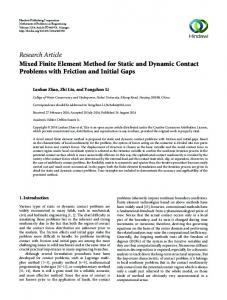


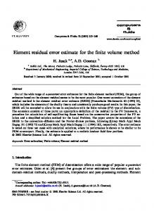


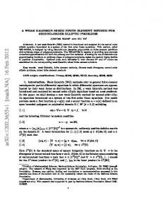

![[hal-00612473, v1] A mixed finite element method for ...](https://m.moam.info/img/260x300/hal-00612473-v1-a-mixed-finite-element-method-for-_5ba02924097c47277e8b45c9.jpg)