A Branch-and-Cut Approach for a Generic Multiple-Product Assembly-System Design Problem Wilbert E. Wilhelm • Radu Gadidov Department of Industrial Engineering, Texas A&M University, TAMUS 3131, College Station, Texas 77843-3131, USA Fort James Corporation, Deerfield, Illinois, 60015, USA
[email protected] _____________________________________________________________________________________ This paper presents two new models to deal with different tooling requirements in the generic multipleproduct assembly-system design (MPASD) problem and proposes a new branch-and-cut solution approach, which adds cuts at each node in the search tree. It employs the facet generation procedure (FGP) to generate facets of underlying knapsack polytopes. In addition, it uses the FGP in a new way to generate additional cuts and incorporates two new methods that exploit special structures of the MPASD problem to generate cuts. One new method is based on a principle that can be applied to solve generic 01 problems by exploiting embedded integral polytopes.
The approach includes new heuristic and
preprocessing methods, which are applied at the root node to manage the size of each instance. This paper establishes benchmarks for MPASD through an experiment in which the approach outperformed IBM's Optimization Subroutine Library (OSL), a commercially available solver. (Programming:Integer,Cutting Planes; Production Scheduling: Flexible Manufacturing Line Balancing) _____________________________________________________________________________________
1. Introduction To serve the specialized demands of customers in today’s highly competitive marketplace, most manufacturers assemble a variety of products, each in relatively low volume. In addition, the advancement of technology has initiated a trend in which product life cycles are becoming shorter. These and other competitive forces require manufacturers to design and redesign assembly systems frequently, so there is a widespread need for improved quantitative methods. This paper describes a new branch-and-cut approach for the generic multiple-product assembly system design (MPASD) problem. The objective is to minimize the total cost of a system design,
1
including the variable cost of assembly operations and the fixed costs of activating assembly stations, purchasing machines, and providing tools. The problem is to prescribe the number of stations, the type of machine to be located at each station, the tooling to be provided at each machine, and the operations to be assigned to each machine. Each operation can be performed on any one of a (perhaps singleton) set of alternative machines and must be assigned to some machine at some station in accordance with precedence relationships. An appropriate set of tools must be provided at each machine to perform assigned operations. Each tool incurs a purchase cost and requires a certain storage space at a machine. Each machine has a finite time availability (i.e., capacity) and finite tool-storage space. The system design must provide sufficient capacity to assemble a specified set of products over the planning horizon. The purpose of this paper is to present two new models, a branch-and-cut solution approach based on several new families of inequalities, and computational evaluation to establish benchmarks for MPASD. Our solution approach can be applied, with minor modifications, to both models. It consists of preprocessing at the root node and a branch-and-cut implementation that adds cuts at each node in the branch-and-bound (B&B) search tree. We generate cuts using the facet generation procedure (FGP) (Parija et al. 1999). In addition, we use the FGP in a new way to generate additional cuts and propose two new methods for generating strong cutting planes by exploiting special structures of the MPASD model. One of these new cut-generating methods is based on a principle that can be applied to solve generic 0-1 problems.
Strong cutting planes are used to tighten the linear representation of the convex hull,
conv(¤) , of feasible integer solutions, ¤ , to facilitate solution of an integer program using linear programming.
The term "strong cutting planes" describes valid inequalities that represent high-
dimensional faces of conv(¤) .
The strongest possible cutting planes, which are of dimension
dim( conv(¤) )-1, represent facets of conv(¤) and provide a complete description of conv(¤) . The Type I assembly line balancing (ALB) problem assigns tasks to a series of identical stations, minimizing the number of stations while observing task precedence relationships and a cycle time requirement (Baybars 1986). A number of studies have focused on the ALB problem and specialized
2
B&B algorithms have been shown to solve selected test problems effectively (e.g., Assche and Herroelen 1979, Johnson 1988, Hackman et al. 1989, Hoffmann 1992, Scholl 1995, Ugurdag et al. 1997, and Scholl and Klein 1997). Assembly system design (ASD) is an extension of ALB in which a robot or other type of “machine” must be assigned to each station, so stations may not be identical.
Each task may be
performed by a set of alternative machine types, and selecting the type of machine to locate at each station entails an additional level of combinatorics, making ASD more challenging than ALB. Task precedence relationships and a cycle time requirement must still be observed. Pinnoi and Wilhelm (1997a) proposed a hierarchical family of models with the goal of dealing with a variety of ASD problems by exploiting the embedded ALB polytope that is common to a variety of formulations. This paper extends the family of models envisioned by Pinnoi and Wilhelm. The single-product ASD (SPASD) problem is typically formulated with the objective of minimizing total cost (e.g., Ghosh and Gagnon 1989, Graves and Lamar 1983), since the design with the minimum number of stations need not minimize cost. Wilhelm (1999) developed a column-generation approach to the SPASD problem.
His approach prescribes the sequence for performing assembly
operations, explicitly addressing tool changes, which, for example, affect the productivity of some robotic assembly systems. Other research has proposed cutting-plane methods for the SPASD problem. Kim and Park (1995) addressed a version of the SPASD problem associated with robotic lines. They assigned tasks, parts, and tools to robotic cells (stations) with the objective of minimizing the total number of cells activated. Their cut-and-branch algorithm included preprocessing and added violated cover cuts (Nemhauser and Wolsey 1988) — all at the root node. Pinnoi and Wilhelm (1998) devised a branch-and-cut approach that employed specialized preprocessing methods. They showed that the node-packing polytope is a relaxation of the ALB polytope and generated a set of cuts based on this relationship. Pinnoi and Wilhelm (1997b) proposed a related approach to the workload-smoothing problem, a variation of ALB that minimizes the maximum idle time on any station, “smoothing” workloads assigned to stations. They generated violated clique and cover
3
inequalities associated with an intersection graph, which they formed from precedence and cycle-time constraints. This prior work demonstrated the effectiveness of using the node-packing relaxation. In contrast, our model incorporates tooling requirements, and we develop strong cutting planes by exploiting special structures that result. Neither tooling requirements nor these new cut-generating methods were considered by Pinnoi and Wilhelm (1997b, 1998). Gadidov and Wilhelm (2000) recently devised a new branch-and-cut approach for the SPASD problem. Their approach, which consisted of a heuristic, preprocessing techniques, and two types of cutting-planes, outperformed OSL in solving a set of test problems. The current paper extends these heuristic and preprocessing techniques to address multiple products and tooling requirements. It also proposes entirely different methods for generating strong cuts. Gadidov and Wilhelm (2000) devised one type of cut based on the time required to complete two tasks that are not related through precedence relationships and incorporated the facet-generation procedure (FGP) (Parija et al. 1999). They added cuts of the former type at the root node and those of the latter type at other nodes in the search tree. The current paper employs the FGP, but its primary contributions include a new way to implement the FGP to generate additional cuts and two new methods for generating cuts based on special structures of the MPASD problem that were not incorporated in the earlier SPASD model. The FGP computes facets of an underlying polytope  , which must be selected so that a subproblem involving a linear objective function can be optimized effectively over it. Parija et al. (1999) applied the FGP to a single constraint so that  was a knapsack polytope and the subproblem can be solved in pseudopolynomial time. Given a fractional solution to the linear relaxation of an integer program, f* (an n vector where n is the number of decision variables in the relaxed problem), the FGP computes the coefficients of a hyperplane, H , that represents a facet of  and separates f* from  . The FGP uses column generation to solve the following linear program (LP): Problem (P): z* = min {åx Î ext  ax | åx Î ext  ax x = f* ; ax ³ 0, x Î ext  }.
4
Here, ext  is the set of extreme points of  , each of which is represented by an n vector, x. The subproblem prices out nonbasic columns, generating the column x Î ext  with the most negative reduced cost. If this reduced cost is nonnegative, the LP optimality criterion is satisfied and the current basis, B * , which is composed of n columns x Î ext  , is optimal. The n vector of coefficients that define the gradient of H , w*, may be determined by solving w* B * = 1. H = { x : w* x £ 1, x
Î ¡ n } supports the n linearly independent points (columns that comprise B * ) so that it represents a facet of
 . Further details may be found in Parija et al. (1999), who proposed the FGP and
demonstrated its efficacy solving 0-1 problems in MIPLIB, and in Gadidov and Wilhelm (2000), who gave an intuitive description of the FGP and incorporated it in an approach for the SPASD problem. The multiple-product ASD (MPASD) problem has received relatively little attention (Ghosh and Gagnon 1989). Variations have been addressed by Lagrangian relaxation (Kuroda and Tozato 1987), B&B (Pinto et al. 1983), dynamic programming (Chakravarty and Shtub 1986), mixed integer programming (Peters 1991), integer programming combined with queueing models (Lee and Johnson 1991), and column generation (Kimms 1998).
Graves and Redfield (1988) enumerated feasible
workstation designs and prescribed MPASD by solving a shortest-path problem. We have organized the body of this paper in four sections. In the next section we introduce notation and our mathematical formulations of two versions of the MPASD problem. Section 3 describes our solution approach. We discuss implementation issues, test problems, and computational results in Section 4. The last section offers final remarks and conclusions.
2. Model Formulation As the ALB model is a generic representation of line-balancing issues, our models are generic representations of MPASD. These models may be applied in a variety of settings, including robotic assembly of airframes e.g., Huber (1984), assembly of automotive subassemblies (e.g., Graves and Redfield 1988) and assembly of electronic products (e.g., Nof et al. 1997).
5
We adopt the traditional approach, combining the operation precedence relationships for the set of products, P , into one digraph (McCaskill 1972). In this digraph, each node represents an operation
o Î O that is required to assemble a subset of products Po Í P . Analogous to the cycle-time constraint that must be observed in SPASD, machine availability (i.e., capacity) must be observed in MPASD. This more general restriction is needed because products may be produced in different volumes and, thus, have different impacts on capacity. This section presents models for two variations of MPASD that deal with different tooling requirements (e.g., Stecke 1983, Graves and Lamar 1983, Ammons et al. 1985, Kim and Park 1995, and Nof et al. 1997). These variations represent typical, practical requirements, and we have designed our cutgenerating methods to exploit the resulting structures. One set of assumptions is common to both of our models. We assume that all parameters are known with certainty: (a) f s , the fixed cost of activating station s Î S ; (b) cm , the fixed cost of machine type
m Î M ; (c) Am , the time availability of machine m ; (d) Bm , the tool-storage space at machine m; (e) c~l , the fixed cost of providing tool type l Î L ; (f) bl , the storage space required by tool type l ; and (g) V p , the production volume for product p Î P . We assume that operation o Î O is completely specified, including the subset of products that require it, Po ; the set of operations that immediately precede it in the precedence digraph, IPo ; the set of associated tools Lo Í L ; the set of alternative machines that can perform it, M o ; and its processing time on each m Î M o , tmo , which incurs variable cost vmo . We now summarize notation. Indices
l m o p s
(l Î L ) (mÎ M ) (o ÎO ) ( pÎ P) (sÎS )
= tool type = machine type = operation = product type = station
Parameters Am = time availability of machine type m
(hours over the planning horizon)
Bm
(square inches or number of slots)
= tool space provided on machine type m
6
bl c~l cm fs tmo vmo Vp
= space required by tool l
(square inches or number of slots)
= fixed cost of purchasing a tool of type l
($)
= fixed cost of purchasing a machine of type m
($)
= fixed cost of activating station s
($)
= processing time of operation o on machine type m
(hours / operation)
= variable cost of performing operation o on machine type m
($/operation)
= production volume required for product type p (number of products over horizon)
Sets
IPo
: set of immediate predecessors of operation o
L
: set of tools
Lo M Mo O Ol Om P Po S
: set of tools required to perform operation o : set of machine types : set of machine types to which operation o can be assigned
L = U oÎO Lo
: set of operations : set of operations that require tool l : set of operations that can be assigned to machine type m : set of types of products : set of products that require operation o
( Po Í P )
: set of stations
S = {1,...,| S |}
Binary Decision variables xmos = 1 if operation o is assigned to a machine of type m at station s , 0 otherwise
yms zlms
= 1 if machine type m is assigned to station s , 0 otherwise = 1 if tool l is assigned to a machine of type m at station s , 0 otherwise.
2.1 MPASD1 Formulation Our first model assumes that operation o Î O requires a set of tools, Lo Î L , and that each tool can be used by several operations. MPASD1 explores tradeoffs between alternative operation assignments and the fixed costs incurred for stations, machines, and tooling. For example, instead of assigning operations that require tool l to different stations, and thus requiring the provision of tool l at each of these stations, it may be less costly to explore alternatives that assign all operations that require tool l to the same station.
7
MPASD1 : min Z BP = å å (c m + f s ) y ms + å å sÎS mÎM
å
å V p v mo x mos + å
sÎS oÎO mÎM o pÎPo
å å c~l z lms
lÎL mÎM sÎS
Subject to:
å å x mos = 1
mÎM o sÎS
å ås x
mos
-
mÎM o sÎS
A m yms -
åt
å ås x
mo ' s
³0
o ÎO
(1)
o Î O, o' Î IPo
(2)
m Î M , s ÎS
(3)
mÎM o ' sÎS
x
mo mos
oÎO m
åV
p
³0
pÎPo
zlms - xmos ³ 0
o Î O , m Î Mo , l Î L o , s ÎS
(4)
Bm yms - å bl zlms ³ 0
m Î M , s ÎS
(5)
åy
s ÎS
(6)
lÎL
mÎM
ms
- å ym ( s +1) ³ 0 mÎM
å y m1 £ 1
(7)
mÎM
o Î O , m Î M o , l Î Lo , s Î S
xmos , yms , zlms Î {0,1}
(8)
The objective function minimizes the total cost of the system design, including the variable cost of performing operations and the fixed costs of activating stations, purchasing machines, and providing tools. This model incorporates all logical issues involved in MPASD. Constraint (1) requires each operation to be processed at one station, and constraint (2) invokes operation precedence relationships. These constraints parallel those used in ALB except that operations in the multiple-product case are called tasks in the singleproduct ALB problem. Constraint (3) imposes machine availability (i.e., capacity) limitations and is the multiple-product analog of the ALB cycle-time requirement. The ALB polytope is embedded in MPASD through constraints (1)-(3) so that the types of cuts derived by Pinnoi and Wilhelm (1998) from the relationship between the node-packing and ALB polytopes could be applied to the MPASD. Since the efficacy of the former set of cuts is known, this paper focuses on the set of new cuts that are related to machine availability and tooling requirements.
8
Neither Pinnoi and Wilhelm (1998) nor Gadidov and Wilhelm (2000) dealt with tooling requirements, a central feature of MPASD. Constraint (4) is a stronger formulation for assuring that appropriate tooling is provided for each operation than was proposed in the models of Pinnoi and Wilhelm (1997a). It assures that the set of tools required by operation o , Lo , are assigned to the machine-station ( ms ) combination at which o is assigned, and it permits tool l to be used by all operations that require that tool ( o Î O; l Î Lo ) if all are assigned to the same ms combination. Constraint (5) invokes the tool-area storage limitation at each machine. Constraint (6) assures that station s will be activated before station s + 1 , precluding symmetry. Together, constraints (6) and (7) assure that at most one machine will be located at each station. These
å
constraints improve earlier models, relying on the the sequence {
mÎM
yms }s being non-increasing.
The number of variables in an instance of MPASD1 depends directly on the number of tools, L ; machine types, M ; operations, O ; and stations, S . The number of constraints depends similarly on these parameters as well as on the number of predecessor relationships for each operation, IPo . The number of products, P , does not affect problem size directly. However, as the number of products increases, the number of operations can also be expected to increase, giving rise to additional precedence relationships,
IPo , tooling requirements, Lo , and machine types, Om , to accommodate the additional operations. 2.2 MPASD2 Formulation Our second model assumes that tools are provided in pre-specified tool kits and that any one of several alternative tool kits, each requiring different space and fixed cost, can perform a given operation. However, each tool kit can perform just one operation. For cases in which each operation may require a number of tools, dealing with tool kits may avoid a combinatorial aspect of the problem. This model explores tradeoffs between the cost of tooling and the storage space required. For example, providing costly tool kits that require little space may allow the system to operate with fewer machines and stations.
9
This model is not overly restrictive because, if a tool kit could perform two operations, it may be preferable to combine them for technical reasons (e.g., Donohue et al. 1991). The notation for this model is the same as before, except that l now denotes a tool kit:
l bl c~
= tool kit = space required by tool kit l
(l Î L ) (square inches or number of slots)
= fixed cost of purchasing a tool kit of type l
($)
L
= set of tool kits
(L =
Lo
= set of tool kits that can perform operation o
( Lo Í L )
l
MPASD2 : min Z BP = å å (c m + f s ) y ms + å å å sÎSmÎM
U
oÎO
Lo )
å V p v mo xmos + å å å c~l z lms
sÎSoÎO mÎM o pÎPo
lÎLmÎM sÎS
Subject to: constraints (1)-(3), (5)-(8) and
åz
lms
- xmos ³ 0
o Î O , m Î Mo , s ÎS .
(9)
lÎLo
As in MPASD1 , the objective function minimizes the total cost of system design. Constraints (9) replace (4), ensuring that some tool kit for operation o is assigned to combination ms along with o .
3. Solution Approach This section describes our solution approach, including the heuristic and pre-processing methods, the two new methods for generating strong cuts, and the strategy for implementation, including the new way in which we use the FGP to generate additional cuts. We demonstrate our methods in relationship to
MPASD1 ; they can be adapted easily for MPASD2 . 3.1 Heuristic and Pre-Processing Methods Our heuristic prescribes an upper bound on the value of the optimal solution, and our pre-processing methods determine an upper bound on the number of stations and the earliest and latest stations to which operation o Î O can be assigned.
3.1.1 Heuristic * We devised a simple heuristic to find an upper bound, Z BPH , on the value of the optimal solution, Z BP , of * MPASD1 (i.e., Z BP £ ZBPH ). At each iteration, the heuristic assigns the operation that can “fit” on a
10
station while incurring the least possible cost. An operation is a candidate for assignment if all of its predecessors (if any) have been assigned. Indices of current candidates are maintained in the set J . When no candidate will fit on the current station, the next station, s , is activated. The machine type m assigned to station s is the one that can process a candidate at minimal cost: m Î argmin{ cm ' + of assigning each candidate
å
lÎLo \ Lms
(å
o Î J Ç Om
pÎPo
)
V p vm ' o : o Î J , m ' Î M o }. We determine the cost
to this ms combination using ~ po =
(å
pÎPo
)
V p vmo +
c%l where Lms is the set of tools already assigned to ms . If o cannot be assigned ( m Ï M o ) or
does not fit (due to tool storage and/or availability limitations), ~ p o = ¥ . At each iteration, we assign an p o : o Î J Ç Om } and update J , Lms , and ~ p o appropriately. When no candidate operation from argmin{ ~
will fit on ms (i.e., min { ~ p o : o Î J Ç Om } = ¥ ) we activate the next station as described above.
3.1.2 Pre-Processing Methods We use Z BPH to obtain an upper bound on the optimal number of stations, N opt . This allows us to fix some variables to zero, managing the size of the problem. We note that this bound is not as pivotal as it is in the ALB problem because the optimal MPASD solution does not necessarily use the minimum number of stations. For example, MPASD must determine an appropriate tradeoff between using a larger number of low-cost machines of lesser capability with using fewer higher-cost machines of greater capability. Assuming that N opt stations have been activated, upper and lower bounds on Z BP are: N opt
åf s =1
s
+ N opt min{ cm : m Î M } + å å Vp min{ vmo : m Î M o } + å c%l £ Z BP £ ZBPH oÎO pÎPo
(10)
lÎL
The first term in (10) represents the cost to activate Nopt stations, the second represents the lowest possible cost of purchasing Nopt machines, the third represents the lowest possible variable cost of performing all the operations, and the fourth represents the cost of purchasing all required tools. Re-expressing (10), we can easily obtain an upper bound for N opt from
11
N opt
åf s =1
s
+ N opt min{ cm : m Î M } £ Z BPH - å å Vp min{ vmo : m Î M o }-å c%l . oÎO pÎPo
(11)
lÎL
We used N opt to manage problem size by defining the earliest ( ES o ) and latest stations ( LSo ) to which operation o can be assigned. Let PRos ( SU os ) denote the set of predecessors (successors) of operation o whose earliest (latest) station is s ( s Î S ):
PRos = { o% : o% = predecessor of o and ESo% = s} and SU os = { o% : o% = successor of o and LSo% = s} . Now, ESo and LSo may be found recursively using the following rules:
ESo = min { so : (1) there exists m Î M o , (2) ESo% £ so
for all predecessors o% of o ,
(3) o fits on mso with any predecessor o% Î PRoso (relative to tool-space and availability limitations) }
LSo = max { so £ N opt : (1)there exists m Î M o , (2) LSo% ³ so for all successors o% of o , (3) o fits on mso with successor o% Î SU oso (relative to tool-space and availability limitations) }. We now describe our two new methods for generating strong cutting planes.
3.2 New Methods for Generating Strong Cutting Planes The first type of cut is based on the structure of our MPASD models. The second type is based on identifying an integral polytope that is embedded in a model. Both focus on tooling requirements. We demonstrate the latter type relative to MPASD, but underlying principles can be applied to integer programs in general.
3.2.1 Cuts Based on Tooling Requirements This section describes our new cutting planes, separation problems, lifting procedures, and implementation strategy. Our first new method for generating cuts exploits structures related to tooling constraints (4) or (9). The cuts may be non-trivial (i.e., some cannot be obtained from a single knapsack constraint (5)). Consider a
12
minimal cover inequality associated with L% Í L in constraint (5) for a given machine type m = m0 and station s = s 0 :
åz lÎL%
£ L% - 1 .
lm0 s0
(12)
Given f* = (x* y* z*), a fractional solution to the linear relaxation of MPASD1 including any applicable generated cuts, the most violated inequality of type (12) can be identified by solving the well-known separation problem (Nemhauser and Wolsey 1988):
ì
å (1 - z )u : å b u î
Problem (SP): Min Z SP = í
* lm0 s0
lÎL
l
l l
lÎL
ü ³ Bm0 + 1; ul Î {0,1} , l Î L ý . þ
{
}
* < 1 Problem (SP) identifies the violated inequality L% = l : ul* = 1, l Î L If Z SP
3.2.1.1 Cutting Planes In addition to the strong cutting planes that may be obtained by lifting cover inequalities (12), a new type of cut may be derived from minimal cover L% in inequality (12) by considering a relationship between z lm0 s0 and x m0os0 decision variables induced by tooling requirements. Let O% ( Í O ) be the set of all
operations that require some tool from set L% , so that O% = { o Î O : $ l Î L% such that o Î Ol } . That is, each operation o Î O% requires at least one tool l Î L% . Note that each tool l Î L% may be required by a number of operations o Î O% . From (12), not all the tools in L% can be assigned to machine type m0 . It follows that not all of the operations in O% can be assigned to machine type m0 , so
åx oÎO%
m0 os0
£ O% - 1
(13)
is an induced relationship, a cover that is valid for MPASD1 . The next subsection describes a separation problem to identify the most violated minimal cover (14) in which K% Í O% :
åx
oÎK%
m0 os0
£ K% - 1 .
13
(14)
3.2.1.2 Separation Given f* = (x* y* z*), L% , and the associated O% , the most violated inequality of type (14) may be found by solving a separation problem that is a set covering (SC) problem of the form:
å (1-x o
Problem (SC): Z SC = min {
* m0 os0
ÎO%
) wo :
åa o ÎO%
lo
~
wo ³ 1 , l Î L% ; wo Î {0, 1}, o Î O }
in which al o = 1 if l Î L% , 0 otherwise. The set-covering constraints assure that Problem (SC) will * < 1 , the optimal solution to prescribe a subset of operations that require all tools in set L% . If Z SC
Problem (SC) defines the inequality of type (14) that is most violated by the current fractional solution f*
{
}
= (x* y* z*), giving the minimal cover K% = o : wo* = 1, o Î O% . We used the greedy heuristic to solve Problem SC (Nemhauser and Wolsey 1988). At each of its iterations, this heuristic accepts the column that satisfies the largest number of uncovered rows per unit cost. It stops when accepted columns cover all rows. The greedy heuristic is not new, but this application of the set-covering problem is, to our knowledge.
3.2.1.3 Lifting Inequality (14) may be strengthened by lifting with respect to variables x m0os0 for o Î O% \K% as follows. First, we note that the greedy heuristic solution to Problem (SC) is “minimal” in the sense that, for any proper subset I% of K% ,
U L% iÎ%I
o
¹ L% . If o Î O% \K% is such that, for any subset I% with I% = K% - 1 , L%o U L%o = L% , iÎ%I
where L%o = L%
IL
o
is the subset of tools in L% required by operation o ,
åx
kÎK%
m0 os0
+ xm0os0 £ K% - 1
(15)
is also a valid inequality for MPASD1 . This logic can yield completely non-trivial valid inequalities for
MPASD1 as shown by the following example.
14
Example. Given f* = (x* y* z*), m0 , and s0 , assume that Problem (SP) identifies the minimum cover
L% = {l1 , l2 , l3} so that these three tools require storage space that is larger than the space available on machine m0 . A valid inequality of type (12) is thus given by set of operations O% =
{o1 , o2 , o3 } ;
åz lÎL%
£ 2 . Assume that the associated
lm0 s0
that L o1 = {l1 , l 2 }, Lo2 = {l2 , l3 } and Lo3 = {l1 , l3 } ; and that,
without loss of generality (wlog), the fractional solution to the linear relaxation satisfies
x m* 0o1s0 £ x m* 0 o2 s0 £ x m* 0o3s0 . The greedy heuristic yields the feasible solution éë wo1
wo2
wo3 ùû = [0 1 1] , which is also
optimal in this case, so that K% = {o2 , o3 } Ì O% = {o1 , o2 , o3 } ; and inequality (14) becomes
x m0o2 s0 + x m0o3s0 £ 1 .
(16)
We may select I% = {o2 } Ì K% = {o2 , o3 } since I% = K% - 1 and L%o1
U L%
o
oÎI%
= {l1 , l2 }
U
{l2 , l3} =
L% = {l1 , l2 , l3} where o1 Î O% \ K% . Inequality (16) may be lifted with respect to x m0o1s0 to obtain a valid inequality of type (15):
x m0o1s0 + x m0 o2 s0 + x m0o3 s0 £ 1.
(17)
We note that (17) is a valid inequality, even though assigning operation o1 Î O% \ K% along with operations in set K% does not exceed the capacity of machine type m0 as invoked by an inequality of type (3):
Am0 -
åV t
pÎPo1
p m0 o1
-
åV t
pÎPo2
p m0 o2
3.2.1.4 Additional Cutting Planes
15
-
åV t
pÎPo3
p m0 o3
³ 0.
Instead of starting with a minimal cover (12) associated with constraint (5), we could begin with a minimal cover of type (14) associated with constraint (3). Starting with inequality (14) and invoking relationships induced by tooling requirements, we obtain a new cut in terms of z lm0 s0 variables. For each o Î O% let &&& Lo = L \
U
Lo denote the set of tools that are required by o and not by
o 'ÎO , o '¹ o
any other operation o ' Î O \ {o} , and assume that none of the sets &&& Lo is empty. From (13), not all the operations in O% can be assigned to machine type m0 , and it follows that not all the tools in
U &&&L
oÎO%
o
can be
assigned to machine type m0 , so an induced relationship that is valid for MPASD1 is given by
ååz
Lo oÎO% lÎ&&&
lm0 s0
£ å &&& Lo - min{ &&& Lo : o Î O% } . oÎO%
3.2.2 Generating Cuts Based on Embedded, Integral Polytopes. Our second new method is based on identifying an embedded integer polytope and lifting over it. The traditional method lifts over the knapsack polytope (e.g., Nemhauser and Wolsey 1988). One advantage of our method is that it lifts by optimizing an LP in polynomial time. A second advantage is that the integer polytope is defined by a number of constraints and may be expected to provide a tighter relaxation of the convex hull of feasible integer solutions than would, say, a single knapsack polytope. We begin this subsection by introducing several claims and a lemma for MPASD1 and an equivalent lemma for MPASD2 . Proofs are given in the Appendix. Subsequently, we describe how the integer polytopes can be used in lifting to generate strong cuts.
3.2.2.1 Embedded Integer Polytopes Lemma 1 establishes the integrality of embedded polytope Â(1) :
(
zT ) :
Lemma 1. The polytope Â(1) = { x T , n
åå
s =1 mÎM
S
xmos +
å åx
mo ' s
n = 1,..., S - 1 , o Î O , o ' Î IPo
£1
s = n +1 mÎM
16
(18)
xmos - zlms £ 0
o Î O , m Î M o , l Î Lo , s Î S
(19) -x £ 0
(20)
–z £ 0
(21)
z £ 1 } is integral.
(22)
Inequalities (18) represent an alternative way of formulating precedence relationships (2), inequalities (19) reiterate inequalities (4), and inequalities (20)-(22) arise in the linear relaxation of binary restrictions (8). A relaxation of MPASD1 , the set of inequalities (18)-(22) admit all solutions that are feasible with respect to (1)-(8) and others as well. For example, (18)-(22) do not assure that each operation is assigned to a single
ms combination as does (1) so that an operation can be unassigned or, in certain cases, assigned to two stations. In addition, inequalities (18)-(22) do not invoke machine-availability limitations (3) or tool-holding capacities (5) and do not require a single machine to be located at each station (6)-(7). Using graph theory, Chaudhuri et al. (1994) proved that the polytope defined by (18) and (20) is integral (see also Ugurdag et al. 1997). We employ an alternative proof strategy and deal with inequalities (19), (21), and (22) as well. First, we introduce some new notation:
n
= n x + nz = total number of variables
nx nz ¤
number of xmos variables
(for o Î O, m Î M o , s Î S )
number of zlms variables
(for o Î O, l Î Lo , m Î M o , s Î S )
set of integer points that are feasible with respect to (18)-(22).
We define n unit vectors, each of dimension n : e mos ( e lms ) is an n vector of zeroes except it has 1 in the unique position determined by index mos ( lms ). We define an agreeable assignment as one that satisfies inequalities (18) with each operation assigned to at most one ms combination. We assume that operation precedence relationships are consistent; that is, if operation o is a predecessor of o ' and if o ' is a predecessor of o " , then o is a predecessor of o " . For example, the assembly tree in which each operation has at most one successor is consistent.
17
Our first claim implies that each extreme point in Â(1) (i.e., each extreme point in conv(¤) (where
conv(¤) Í Â(1) )) is formed by the intersection of n linearly independent, binding inequalities (Bazaraa et al. 1990) defining Â(1) and conv(¤) , respectively. Claim 1 dim( Â(1) ) = n and dim( conv(¤) ) = n . Each extreme point of Â(1) is formed by a subsystem of n linearly independent inequalities in (18)(22) that hold at equality. We prove Lemma 1 using a strategy that shows that each feasible subsystem forms an extreme point that is integral, so that Â(1) is integral. If more than n inequalities hold at equality at an extreme point, n linearly independent inequalities imply each of those in excess, whether it is essential or redundant. We show that, at each extreme point, each of the n variables is related to a unique binding inequality and that this set of equalities is linearly independent. We begin by considering feasible subsets that require xmos = 0 for all mos combinations. Claim 2 Each subsystem formed by fixing two types of inequalities to equalities (a) all n x inequalities (20) and (b) for each lms , select an inequality of type (21) fixing zlms = 0 or of type (22) fixing zlms = 1 gives n linearly independent, binding inequalities that define an extreme point, which is integral.
(
The null solution x T ,
z T ) = ( 0T , 0T ) is a special case in which inequalities (20) and (21) are all fixed
at equality. MPASD1 assumes that each operation requires a set of tools and that each tool may be used by more than one operation. Claim 2 highlights the fact that each zlms is constrained on the range
zlms = max oÎO:lÎLo {xmos } £ zlms £ 1, in which the operations that require tool l determine the lower bound; and inequality (22), the upper bound. Next, we consider Dmos , the index set of the subset of constraints (18) in which a selected variable,
xmos , has the coefficient 1. If xmos is set to 1, each of the other variables with coefficient 1 in at least one of these constraints must be set to 0. Variables associated with subset Dmos include:
18
(i) xmos two types of variables incorporated in the first summation of (18) (ii) xm ' os , which assigns operation o to alternative machine m ' Î M o \ {m} at station s , and (iii) xm ' os ' , which assigns operation o to some machine m ' Î M o at station s ' (1 £ s ' £ S - 1, s ' ¹ s ), variables associated with each immediate predecessor o ' Î IPo of operation o (iv) xm ' o ' s ' , which assigns predecessor o ' Î IPo to some machine m ' Î M o ' at a downstream station s ' > s , two types of variables that have coefficient 1 in rows where xmos is in the second summation (v) xm "o " s " , which assigns immediate successor operation o Î IPo " to some machine m " Î M o " at an upstream station s " < s , and (vi) xm ' os ' , which assigns operation o to some machine m ' Î M o at another station 2 £ s ' £ S , s ' ¹ s . We now characterize extreme points associated with a selected subset Dmos . Claim 3 Each subsystem formed by fixing four types of inequalities to equalities (a) the selected subset Dmos of inequalities (18), (b) all nz inequalities (20) except for the one associated with xmos , (c) inequality (22) for all tools l Î Lo used by combination mos , and (d) for each lms combination not included covered by (c), select an inequality of type (21), fixing zlms = 0, or of type (22), fixing zlms = 1, gives n linearly independent, binding inequalities that define an extreme point, which is integral. Claim 3 may be readily extended to deal with all agreeable assignments. Claim 4 Each subsystem formed by fixing four types of inequalities to equalities (a) selected subsets Dmos of inequalities (18) associated with mos combinations in the agreeable assignment, (b) all nz inequalities (20) except for the ones associated with the xmos in the agreeable assignment, (c) inequality (22) for all tools l Î Lo used by combinations mos in the agreeable assignment, and (d) for each lms combination not included covered by (c), select an inequality of type (21), fixing zlms = 0, or of type (22), fixing zlms = 1, gives n linearly independent, binding inequalities that define an extreme point, which is integral. We now extend Claim 4 to deal with extended agreeable assignments for which extreme points that represent feasible integer solutions allow an operation to be assigned to two stations. This possibility arises because the first summation in inequality (18) is for stations 1 £ n £ S - 1 . Thus, it is feasible for xmo|S | = 1
19
even when xmon = 1. Upstream assignment mon is limited only by assignments of predecessors o ' Î IPo . Assignment mo | S | is limited only by the assignments of immediate successors o " where o Î IPo " . Claim 5 If each immediate predecessor of combination mos , o ' Î IPo , is either unassigned or assigned agreeably (i.e., at station s ' where s ' < s , given mos ) and each successor o " (i.e., where o Î IPo " ) is unassigned or assigned to station S , then xmo S may also be set to 1 for any m Î M o in addition to xmon = 1. This revises certain inequalities of two types, (b) and (d), that are fixed to equalities in Claim 4: (b’) instead of inequality (20), use inequality (19) for each designated combination mo | S | for any m Î M o (d’) instead of inequality (21) or (22), use inequality (22) for all tools l Î Lo used by combination mo | S | . This gives n linearly independent, binding inequalities that define an extreme point, which is integral. Claims 6 and 7 and Corollary 1 show that Â(1) has no fractional extreme point solution. Claim 6 If nxf variables of type xmos are set to fractional values (1 £ nxf £ nx ) , they cannot be associated with a set of nxf linearly independent binding inequalities of type (18). The implication of Claim 6 is that no set of n linearly independent, binding inequalities intersect to form a fractional extreme point. Note that a fractional xmos variable could be related to one of the Lo inequalities of type (19), but then one of the associated zlms variables for l Î Lo could not be related to an independent, binding inequality because zlms = xmos for all l Î Lo so that zlms could not be related to an inequality of type (21) or (22). Corollary 1 identifies the important result that combination os can be assigned to at most one machine m Î M o . It limits both integral and fractional solutions. Corollary 1 If 0 < xmos £ 1 , xmos ' for m ' Î M o \ {m} may be associated with a binding inequality that is linearly independent of others if and only if inequality (20) holds at equality, that is xm ' os = 0. Now, consider values of zlms that are not determined by fixing an inequality of type (19), (21), or (22). Claim 7 If variable zlms is assigned a fractional value on zlms = max oÎO:lÎLo {xmos } < zlms < 1, it cannot be associated with a binding inequality. Because of the relationships imposed by inequalities (18), relatively few subsystems must be considered in the proof of Lemma 1. In addition, a related integral polytope is defined by Corollary 2. Corollary 2 Inequalities (19)-(22) and
20
n
S
å å xmos + å
s =1mÎM
n = 1,..., S , o Î O , o'Î IPo ,
å x mo 's £ 1
s = n +1 mÎM
(23)
in which the second summation is vacuous when n = S , define an integral polytope. Inequality (23) allows n = S in inequalities (18), assuring that each operation will be assigned to at most one ms combination, precluding the assignments described in Claim 5. In MPASD2 , each operation requires one tool kit to be selected from a set of alternatives and each tool kit may be used by only one operation. The polytope that corresponds to Â(1) replaces (19) with (9).
(
Lemma 2 The polytope Â(2) = { x T ,
z T ) : (18), (9), (20), (21), and (22)} is integral.
The proof of Lemma 2 relies on Claim 8, which is the MPASD2 version of Claim 5 for extended agreeable assignments. Otherwise, the proof follows that of Lemma 1 so that details are not presented. Claim 8 Each subsystem formed by fixing six types of inequalities to equalities (a) selected subsets Dmos of inequalities (18) for mos combinations in the extended agreeable assignment, (b’) inequality (9) for each designated combination mo | S | for any m Î M o , (b) all nz inequalities (20) except for the ones specified in (a) and (b'), (c) inequality (9) for one selected tool l Î Lo used by each mos combination in (a) and (b'), (c') inequality (21) for each tool required by each mos combination in (a) and (b') that is not selected in (c): l ' Î Lo \{l} , and (d) for each lms combination not covered by (c) and (c'), select an inequality of type (21), fixing zlms = 0, or of type (22), fixing zlms = 1, gives n linearly independent, binding inequalities that define an extreme point, which is integral. Finally, an integral polytope is also defined if inequalities (18) are tightened as described in Corollary 2. Again, details of the proof are omitted. Corollary 3 Inequalities (9) and (20)-(23) define an integral polytope.
3.2.2.2 Generating Cuts Now, fix a m0 Î M and s0 Î S and assume that a valid inequality for MPASD1 is given by
åa z lÎL%
l lm0 s0
£ b ym0 s0 ,
21
where L% Í L such that, for each o Î Om0 , L% Ç Lo ¹ Æ. In an optimal solution, no station can be activated without assigning at least one operation to it. Thus,
a~ y m0 s0 £ å a l z lm0 s0 ~ lÎL
is also a valid inequality, in which a~ = min {
åa
~ lÎL
I Lo
l
(24)
: o Î O m0 }.
Using Lemma 1 for MPASD1 (or Lemma 2 for MPASD2 ), we can improve (24) by lifting with respect to variables x m0os0 , o Î Om0 over embedded polytope Â(1) ( Â(2) ). So, assume that
a% ym0 s0 £ å a l zlm0 s0 - å bo xm0os0 lÎL%
oÎO%
(25)
is an inequality obtained from (24) by lifting with respect to variables x m0os0 , o Î O% , where O% is a subset of O , and b o > 0 for all o Î O% . Moreover, let o Î Om0 \O% and let the lifting problem associated with variable x m0os0 be defined as
b o' = min {
åa z lÎL%
l lm0 s0
-å bo% xm0os% 0 : x Î Â(1) , xm0os0 = 1 } . o%ÎO%
The LP solution to this problem prescribes binary values for x decision variables and the lifting coefficient b o' .
~ , another inequality that is valid for MPASD is given by If b o' > a 1
a% ym0 s0 £ å a l zlm0 s0 - å bo xm0os% 0 - ( bo' - a% ) xm0os0 lÎL%
(26)
o%ÎO%
since the integral polytope associated with inequalities (2)-(5) is a subset of Â(1) . A similar argument holds for MPASD2 , and we omit details. Lifted inequalities (25) and (26) translate precedence relationships for operations to tools. The following example demonstrates the cut-generating procedure described in this section (3.2.2). Example For simplicity, assume there is only one machine, L = {l1 , l2 , l3 } , O = {o1 , o2 , o3 } , and o2 must be performed after o1 ; and o3 , after o2 . Let s0 = 1 and assume that inequality (5) is
22
2 zl1s0 + 3 zl2 s0 + 5 zl3 s0 £ 7 ys0 . In this case, (24) becomes 2 ys0 £ 2 zl1s0 + 3 zl2 s0 + 5 zl3 s0 . Now, one may lift with respect to xo2 s0 in the following manner: min{2 zl1s0 + 3 zl2 s0 + 5 zl3 s0 : xo2 s0 = 1, x Î Â(1) } = 5 since xo2 s0 = 1 implies xo1s0 = 1 (so zl1s0 = zl3 s0 = 1 from (4)). Therefore, 2 ys0 £ 2 zl1s0 + 3 zl2 s0 + 5 zl3 s0 - 3 xo2 s0 is also a valid inequality for MPASD1 . We now describe our implementation strategy.
3.3 Implementation Strategy We apply our heuristic and preprocessing methods at the root node. The heuristic determines an upper bound, Z BPH , on the value of the optimal solution. In turn, our preprocessing methods use Z BPH to determine an upper bound on the number of stations, Nopt, as well as the earliest ( ESo ) and latest ( LSo ) stations to which operation o Î O may be assigned. These bounds limit the size of each instance. * We solved MPASD1 ( MPASD2 ) to obtain the optimal binary solution, Z BP , using the branch-
and-cut capabilities of OSL. To implement branch and cut, OSL uses its supernode routine to manage cuts generated by user-supplied routines. OSL’s supernode routine (IBM 1995) invokes pre-processing methods (e.g., bound tightening and coefficient reduction using probing techniques) at nodes of a B&B search tree to strengthen the linear relaxation. It is called “supernode” because it may fix several variables while analyzing one node in the search tree; in this way it is comparable to the analysis done at a number of nodes in the traditional search tree. It implements branch and cut, adding certain inequalities, for example, derived from the implication lists that result from probing. It also calls a routine through which the user may add generated cuts. Supernode manages cuts; for example, it may discard an
23
inequality if it becomes nonbinding. Supernode also employs a heuristic that attempts to determine a feasible solution, and it may eliminate cuts after invoking its heuristic. Our routines apply the FGP to individual knapsacks defined by inequalities (3), generating inequalities of type (14) using separation Problem (SC), and apply Lemma 1 for MPASD1 (Lemma 2 for MPASD2 ) to lift inequality (24). We applied the solutions prescribed by the FGP in several ways. We used FGP solutions to generate cuts associated with inequalities (3) directly. In addition, we used FGP solutions in a new way, lifting the vectors that comprise an optimal basis for Problem P to obtain cover inequalities (12) and (14), which were subsequently strengthened by our new lifting methods.
4. Computational Evaluation To establish computational benchmarks, we ran a set of tests on an IBM RISC 6000 model 550 using OSL release 3. We are aware of no other special-purpose algorithms to solve MPASD1 and MPASD2 , so we compared our approach with OSL using its capable supernode routine to implement B&B. Thus, the only difference between the two approaches is that one employs our cut-generating methods. This section describes the set of random test instances we generated as well as test results.
4.1 Test Instances We designed an experiment with four factors to gain insight into the influence they have on the run time to solve MPASD1 and MPASD2 . Resource limitations did not allow us to replicate each treatment; however, experiments of this design are commonly used to evaluate mathematical programming algorithms. The factors we considered and the levels for each were: Factor (1) machine availability (2) precedence relationships (3) number of alternative machine types (4) number of products
24
Levels 4000 (4, 7) 2 3
6000 (3, 5) 4 4
6
We defined the levels for factor (1) by Am = ci / rm for i = 1, 2 for each m Î M . We specified
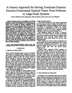
c1 = 4000 and c2 = 6000 and drew rm randomly from U[0.5, 1.0]. The levels for factor (3) were 2, 4, and 6, and those for factor (4) were 3 and 4. The levels for factor (2) were contingent on factor (4). Instances that involved 3 products employed precedence digraphs with either 4 (Figure 1) or 7 (Figure 3) rows of nodes. Instances that involved 4 products employed precedence relationships with either 3 (Figure 2) or 5 (Figure 4) rows of nodes. We used the precedence digraphs in Figures 1-4 for both MPASD1 and MPASD2 instances. Each node in these figures represents an operation, an arc represents an immediate precedence relationship, and the number(s) within each node indicate the product(s) that require the associated operation. We designed digraphs 1 and 2 (3 and 4) so that about 50% (75%) of all possible arrows from one layer to the next were generated, and about 50% (75%) of the operations are common to two or more products. Precedence relationships are relatively dense, contributing to the difficulty of the instances. We used the same factors in testing model MPASD2 , generating a set of 24 instances of
MPASD1 and another 24 of MPASD2 . We generated tooling constraints in MPASD1 so that 30%,
Figure 1: Precedence Diagram 1 for MPASD Problems
25
Figure 2: Precedence Diagram 2 for MPASD Problems
Figure 3: Precedence Diagram 3 for MPASD Problems
26
Figure 4: Precedence Diagram 4 for MPASD Problems
60%, and 10% of the operations require 1, 2, and 3 tools, respectively, and 60%, 30%, 6%, and 4% of the tools were required by 1, 2, 3, and 4 operations, respectively. Generated tool-kit constraints in MPASD2 assigned a unique tool kit to each of 10% of the operations and allowed 50%, 30%, and 10% of the operations to select from 1 of 2, 1 of 3, or 1 of 4 tool kits, respectively. Tables 1 and 2 describe our test problems. Each row describes an instance. The first column specifies the model and level of each factor associated with an instance. Notation is self-explanatory, for example, mpasd1/ c1l 4m 2 p3 represents an MPASD1 instance with c1 = 4000, four rows in the precedence digraph, two types of alternative machines, and three products. Other columns give the * number of constraints; number of variables; optimal values for the initial LP relaxation, Z LP ; optimal * * * * * binary solution, Z BP ; and percent gap, %Gap = 100 ( Z BP - Z LP ) / Z BP . We obtained Z BP , the optimal
binary solution to each MPASD1 ( MPASD2 ) instance using the strategy described in Section 3.3. The
27
average %Gap for the 24 MPASD1 instances was 13.75%, and that for the 24 MPASD2 instances was 9.30%. We now describe test results.
4.2 Test Results Tables 3 and 4 summarize test results. Each row describes an instance. The first column specifies the model and level of each factor associated with an instance. Columns 2-4 describe the performance of our approach, giving, respectively, the number of cuts generated during the branch-and-cut tree search, the number of B&B nodes required to find and verify an optimal solution, and the CPU run time (in seconds) for solving the instance. We adopted CPU run time as the primary measure of our approach and the number of nodes required to find and confirm an optimal solution as a secondary measure. Columns 5-6 describe the performance of OSL, giving, respectively, the number of B&B nodes to find and verify the optimal solution and the CPU run time (in seconds). We set a run-time limit of five hours for each instance. Our heuristic and pre-processing methods serve only to manage the sizes of instances, so we document their effects only in columns 2 and 3 of Tables 1 and 2. On average, our heuristic prescribed a solution that was 1 to 2 stations higher than the optimal number of stations. However, even in the few instances in which the heuristic prescribed the optimal number of stations, both our branch-and-cut approach and OSL took some time to find and verify an optimal solution. Our approach was able to solve 46 of these 48 instances within run-time and storage limitations, but OSL was able to solve only 32 instances. On these 32 instances, our approach required, on average, significantly less run time and significantly fewer nodes in the search tree.
28
Table 1: MPASD1 Test Instances Instance Mpasd1/c1 l 4m2p3 Mpasd1/c1 l3m2p4 Mpasd1/c1 l 4m4p3 Mpasd1/c1 l3m4p4 Mpasd1/c1 l 4m6p3 Mpasd1/c1 l3m6p4 Mpasd1/c2 l 4m2p3 Mpasd1/c2 l3m2p4 Mpasd1/c2 l 4m4p3 Mpasd1/c2 l3m4p4 Mpasd1/c2 l 4m6p3 Mpasd1/c2 l3m6p4 Mpasd1/c1 l7 m2p3 Mpasd1/c1 l5m2p4 Mpasd1/c1 l7 m4p3 Mpasd1/c1 l5m4p4 Mpasd1/c1 l7 m6p3 Mpasd1/c1 l5m6p4 Mpasd1/c2 l7 m2p3 Mpasd1/c2 l5m2p4 Mpasd1/c2 l7 m4p3 Mpasd1/c2 l5m4p4 Mpasd1/c2 l7 m6p3 Mpasd1/c2 l5m6p4 * Not optimal
Rows 441 415 738 684 1035 1000 459 433 729 667 1026 1000 838 775 1468 1360 1788 2185 928 805 1528 1585 1888 2065
Variables 423 396 738 702 1080 1026 405 405 720 684 1098 1089 975 1005 1845 1800 2400 2820 1155 1020 1965 2085 2535 2715
* Z LP
358755.800 402261.900 355497.100 361957.800 318314.300 335774.800 358761.600 347605.600 364156.400 310854.300 321218.300 325703.600 729758.700 732501.200 751194.400 698182.000 728098.000 650681.200 770942.400 729075.100 742920.200 654187.500 700416.500 626691.400
* Z BP
448299.311 435740.790 438847.722 428264.502 436693.404 402742.255 417007.557 426133.741 414689.917 409076.253 395627.739 394885.599 832577.857 799873.179 824941.650 781576.445 786504.736 792423.100* 824838.760 762525.201 813259.131 739959.028 799716.174 696597.748
% Gap 19.97 7.68 18.99 15.48 27.11 16.63 13.97 18.43 12.19 24.01 18.81 17.52 12.35 8.42 8.94 10.67 7.43 17.89 6.53 4.39 8.65 11.59 12.42 10.04
It is difficult to generalize the effect of each factor on run time. It appears that increasing machine availability tended to make instances somewhat easier to solve. Increasing the number of alternative machines for each operation from 2 to 4 to 6 tended to increase the number of assignment combinations and the level of difficulty. As expected, results showed that run time increased with the number of operations. Even though model MPASD2 is somewhat tighter than MPASD1 , most larger instances (i.e., those with 5 or 7 layers in their precedence relationships) remained challenging, requiring, on average, more than one hour to obtain an optimal solution.
29
Table 2: MPASD2 Test Instances Instance mpasd2/c1 l 4m2p3 mpasd2/c1 l3m2p4 mpasd2/c1 l 4m4p3 mpasd2/c1 l3m4p4 mpasd2/c1 l 4m6p3 mpasd2/c1 l3m6p4 mpasd2/c2 l 4m2p3 mpasd2/ c2 l3m2p4 mpasd2/c2 l 4m4p3 mpasd2/c2 l3m4p4 mpasd2/c2 l 4m6p3 mpasd2/c2 l3m6p4 mpasd2/c1 l7 m2p3 mpasd2/c1 l5m2p4 mpasd2/c1 l7 m4p3 mpasd2/c1 l5m4p4 mpasd2/c1 l7 m6p3 mpasd2/c1 l5m6p4 mpasd2/c2 l7 m2p3 mpasd2/c2 l5m2p4 mpasd2/c2 l7 m4p3 mpasd2/c2 l5m4p4 mpasd2/c2 l7 m6p3 mpasd2/c2 l5m6p4 * Not optimal
Rows 244 244 378 397 540 559 243 235 396 379 540 550 613 550 928 835 1184 1135 552 565 987 850 1228 1150
Variables 603 666 999 1143 1485 1611 612 639 1143 1035 1557 1566 1605 1260 2475 2115 3285 2940 1470 1380 2580 2130 3375 3060
* Z LP
422046.300 443201.600 415798.900 413535.300 427301.600 382274.100 408345.800 428021.500 405385.600 410771.500 365836.100 399938.600 749766.500 704812.700 758145.000 750197.300 744281.500 691959.800 710704.700 727657.500 701196.600 683543.400 697886.700 693993.100
* Z BP
485713.914 459175.452 473070.047 447119.552 452714.600 442762.028 458761.237 453788.010 436343.744 451910.402 423945.775 441549.025 824602.733 790281.321 823767.762 785682.100 821238.000* 759719.700 819446.214 802395.500 775012.310 797080.400 791351.341 714803.445
% Gap 13.11 3.48 12.11 7.51 5.61 13.66 10.99 5.68 7.09 9.10 13.71 9.42 9.08 10.81 7.97 4.52 9.37 8.92 13.27 9.31 9.52 14.24 11.81 2.91
Our test instances were not large relative to parameters, L , M , O , and S . However, MPASD is challenging because precedence relationships, alternative machines, machine capacities, tooling requirements, and tooling-space limitations interact combinatorially to increase difficulty. As the theory of computational complexity would suggest, run time was related to problem size as measured by the number of decision variables. Instances with fewer than 700 variables tended to be relatively easy to solve. However, OSL (without our new methods) could not solve most problems with over 2000 variables. A few relatively small instances were particularly challenging, while a few of the largest
30
instances were solved easily. The two problems that our new methods did not solve within the run-time limit were the largest MPASD1 instance with 2820 variables and the largest MPASD2 instance with 3285 variables. Table 3: MPASD1 Test Results Branch and Cut Cuts Nodes
Instance
*
OSL *
Mpasd1/c1 l 4m2p3 Mpasd1/c1 l3m2p4
340 15
12 0
CPU (sec.) 165 11
Mpasd1/c1 l 4m4p3 Mpasd1/c1 l3m4p4 Mpasd1/c1 l 4m6p3 Mpasd1/c1 l3m6p4 Mpasd1/c2 l 4m2p3 Mpasd1/c2 l3m2p4 Mpasd1/c2 l 4m4p3 Mpasd1/c2 l3m4p4 Mpasd1/c2 l 4m6p3 Mpasd1/c2 l3m6p4 Mpasd1/c1 l7 m2p3 Mpasd1/c1 l5m2p4 Mpasd1/c1 l7 m4p3 Mpasd1/c1 l5m4p4 Mpasd1/c1 l7 m6p3 Mpasd1/c1 l5m6p4 Mpasd1/c2 l7 m2p3 Mpasd1/c2 l5m2p4 Mpasd1/c2 l7 m4p3 Mpasd1/c2 l5m4p4 Mpasd1/c2 l7 m6p3 Mpasd1/c2 l5m6p4
538 297 2513 2905 74 125 72 430 1286 1116 4922 355 3780 4078 1165 3832 147 201 1300 1057 4143 11051
25 7 54 53 0 7 3 18 52 30 63 7 64 155 27 176 0 0 33 36 81 456
725 345 1520 2837 81 143 79 426 839 841 8866 720 7219 16997 5000 18000** 1496 510 10977 14429 14075 16940
All times are in seconds ** Time or Memory over limit
31
19 0
CPU* (sec.) 145 36
107 26 582 134 0 5 7 66 137 118 239 ** 301 ** 73 ** 5 ** ** ** ** **
1134 446 6375 4400 48 90 201 976 2476 4673 16390 ** 15874 ** 16423 ** 2412 ** ** ** ** **
Nodes
Table 4: MPASD2 Test Results
Instance
Cuts
Mpasd2/c1 l 4m2p3 Mpasd2/c1 l3m2p4 Mpasd2/c1 l 4m4p3 Mpasd2/c1 l3m4p4 Mpasd2/c1 l 4m6p3 Mpasd2/c1 l3m6p4 Mpasd2/c2 l 4m2p3 Mpasd2/c2 l3m2p4 Mpasd2/c2 l 4m4p3 Mpasd2/c2 l3m4p4 Mpasd2/c2 l 4m6p3 Mpasd2/c2 l3m6p4 Mpasd2/c1 l7 m2p3 Mpasd2/c1 l5m2p4 Mpasd2/c1 l7 m4p3 Mpasd2/c1 l5m4p4 Mpasd2/c1 l7 m6p3 Mpasd2/c1 l5m6p4 Mpasd2/c2 l7 m2p3 Mpasd2/c2 l5m2p4 Mpasd2/c2 l7 m4p3 Mpasd2/c2 l5m4p4 Mpasd2/c2 l7 m6p3 Mpasd2/c2 l5m6p4
582 54 717 2249 385 6024 144 65 1244 629 1042 229 866 1540 5344 505 6150 571 292 347 16566 7520 3185 1304
Branch and Cut Nodes CPU* (sec.) 19 259 0 19 52 890 60 2568 19 142 421 3421 2 54 0 40 104 1600 40 842 111 1522 14 250 21 1400 8 1920 159 9104 6 1905 137 18000** 12 1200 0 418 0 400 400 16496 192 14242 36 13946 8 2300
OSL Nodes 52 27 57 121 37 ** 1 0 ** 51 ** 20 31 37 ** 41 ** 52 4 3 ** ** ** 39
CPU* (sec.) 875 423 2045 8921 632 ** 524 126 ** 1729 ** 1210 3200 3781 ** 4218 ** 4734 1920 904 ** ** ** 8732
* All times are in seconds ** Time or Memory over limit
5. Conclusions This paper presents two new models to deal with different tooling requirements in the generic multipleproduct, assembly-system design (MPASD) problem; describes a branch-and-cut solution approach based on several new families of inequalities, and establishes computational benchmarks. Our solution approach can be applied, with minor modifications, to both models. Our approach includes new heuristic and
32
preprocessing methods that manage the size of each instance. It employs the facet generation procedure (FGP) to generate facets of underlying knapsack polytopes. In addition, it uses the FGP in a new way to generate additional cuts and incorporates two new methods that exploit special structures of the MPASD problem to generate cuts. One of our new methods is based on a principle that exploits embedded, integral polytopes and can be applied to solve generic 0-1 programs. This paper establishes computational benchmarks for the MPASD problem by describing an experiment that involved 24 test instances of each of the two MPASD models. Test results show that our method performed particularly well in comparison to OSL; it had better run times on three instances, required fewer nodes in one instance, and posted both better run times and fewer nodes in 40 of the 48 instances.
OSL
performed
somewhat
better
on
two
instances
(mpasd1/c2 l 4m2p3
and
mpasd1/c2 l 3m2p4), which were relatively easy for both approaches, and neither approach was able to solve the two largest instances (mpasd1/c1 l5m6p4 and mpasd2/c1 l7 m6p3 ) within the run-time limit. Increasing levels of factors (1) machine availability and (3) number of alternative machine types for each operation did not affect run time in a consistent way.
However, increasing levels of factors (2),
precedence relationships, and (4), number of products, increased the number of operations and resulted in increased run times. Results indicate that the MPASD problem is amenable to our new cutting-plane methods, even though tooling considerations entail an additional level of combinatorics, making our MPASD problems more challenging than the ASD problems studied by Pinnoi and Wilhelm (1997b, 1998) and Gadidov and Wilhelm (2000). It would be possible to combine our new cut-generating methods with those devised by Pinnoi and Wilhelm (1998), which rely upon relationships between the node-packing and assembly-line balancing polytopes, but focusing on our new cut-generation methods allowed us to assess their efficacy. Test results show that the new methods presented in this paper collectively form a credible solution approach. Future research may, however, investigate the relative efficacy of each applicable family of inequalities, including those based on ASD (Pinnoi and Wilhelm 1998) and MPASD (as described in
33
this paper) as well as those related to more generic problems such as the precedence-constrained knapsack, multiple knapsack, and generalized assignment problem.
Appendix This Appendix presents proofs of Claims, Corrolaries, and Lemmas. Proof of Claim 1: (a) dim( Â(1) ) £ n and dim( conv(¤) ) £ n since both incorporate n decision variables. (b) dim( Â(1) ) ³ n and dim( conv(¤) ) ³ n since each polytope contains n + 1 affinely independent points: (i) one point: (xT, zT) = (0T, 0T)
( )
T , one for each of the nz lms combinations (ii) nz points: (xT, zT) = elms
(iii) n x points: (xT, zT) =
(e
T mos
)
T - å lÎL elms , one for each of n x mos combinations. o
(1)
(c) Combining (a) and (b), dim( Â ) = n and dim( conv(¤) ) = n . Q.E.D. Proof of Claim 2. A basis matrix representing an extreme point of Claim 2 may be composed of rows T (a) -emos for all mos ( n x binding inequalities (20)) T T or elms for each lms (b) -elms
( nz binding inequalities of type (21) or (22))
representing n linearly independent, binding inequalities. Each of these extreme points is integral. Q.E.D. Proof of Claim 3. A basis matrix representing an extreme point of Claim 3 may be composed of rows T (a) emos for combination mos , upon which subset Dmos is defined T for each combination m ' o ' s ' other than mos (b) -em'o's' T for each l Î Lo required by combination mos (c) elms
T T or el'm's' for each l ' Î Lo ' associated with combinations m ' o ' s ' other than mos (d) -el'm's' representing n linearly independent, binding inequalities. Each of these extreme points is integral. Elementary row operations (EROs) can be performed on each row in subset Dmos , adding (or subtracting) the T . Any one of these reduced rows may be used in (a); the appropriate row in (b)-(d) to reduce that row to emos
others are implied by it. Q.E.D. Proof of Claim 4. A basis matrix representing an extreme point of Claim 4 may be composed of rows T (a) – emos for each combination mos associated with the agreeable assignment T (b) -em'o's' for each combination m ' o ' s ' other than combinations mos associated with the agreeable assignment T (c) elms for each l Î Lo required by an mos combination associated with the agreeable assignment T T or el'm's' for each l ' Î Lo ' associated with combinations m ' o ' s ' other than mos combinations (d) -el'm's' associated with the agreeable assignment representing n linearly independent, binding inequalities. Each of these extreme points is integral.
34
Subsets Dmos for each pair of combinations in the agreeable assignment have no rows or columns in common. Elementary row operations (EROs) may thus be performed on each row in each subset Dmos , T as in the proof to Claim 3. adding (or subtracting) the appropriate rows in (b)-(d) to reduce that row to emos
Q.E.D. Proof of Claim 5. A basis matrix representing an extreme point of Claim 5 may be composed of the rows described in the proof of Claim 4 but modified by using T T - elms for each designated combination mo | S | for any m Î M o and l Î Lo (b’) emos T for each l Î Lo associated with combination mo | S | . (d’) elm S
The revised set represents n linearly independent, binding inequalities. Each of these extreme points is integral. Q.E.D. Proof of Claim 6. If nxf = 1, a single fractional xmos cannot make any inequality (18) hold at equality because each has RHS equal to 1. Now, suppose that nxf variables of type xmos are fractional and they appear in n18£ inequalities of type (18), n18= of which hold at equality. Clearly, if nxf < n18= , the rows are linearly dependent. If nxf > n18£ ³ n18= or nxf = n18£ > n18= , (nxf - n18= ) ³ 1 so that the nxf variables cannot be associated with nxf binding inequalities (18). Now, consider three cases in which nxf = n18£ = n18= . (Case 1): If the same nxf variables appear in all n18£ = n18= binding inequalities, EROs can be used to show that these rows are linearly dependent. Thus, in case 1, the nxf variables cannot be associated with
nxf linearly independent, binding inequalities. (Case 2): If the row of (18) in which xmos first appears contains xmos in the first summation, successive inequalities add variables that assign operation o downstream of station s (i.e., at station s ' where s ' > s ) as n increases and/or different predecessors (i.e., o ' Î IPo ) downstream of station s . (Case 3): If the row of (18) in which xmos first appears contains
xmos in the second summation, successive inequalities add variables that assign successors at other stations upstream of station s . In Case 2 or 3, the row in which xmos first appears must contain fewer than nxf fractional variables that cannot add to 1. This is true because each of the other rows contains at least one additional fractional variable and the fractions must add to 1 in each of those rows. If not, the row in which xmos first appears must contain the same set of variables that appear in each of the n18£ = n18= rows and this set of rows is not linearly independent). Q.E.D. Proof of Corollary 1. (Þ)A basis matrix representing an extreme point of Corollary 1 may be composed using the rows of Claim 5, modified by T (a”) – emos for each combination mos where it is desired that xmos be on the range 0 < xmos £ 1 T for each combination m ' os where m ' Î M o \ {m} and it is desired that xm ' os = 0 (b”) -em'o's' The revised subsystem represents n linearly independent, binding inequalities. Each of these extreme points is integral.
35
(Ü) Given 0 < xmos £ 1 , suppose o < xm ' os £ 1 (for m ' Î M o \ {m} ). Claim 6 establishes that both xmos and xm ' os cannot be fractional and inequalities (18) do not allow both to equal 1. Therefore, xm ' os = 0 must hold. Q.E.D. Proof of Claim 7. zlms may only be associated with binding inequalities (19) xmos = zlms (for
o Î O : l Î Lo ), (21) zlms = 0, or (22) zlms = 1 so that, if it is fractional and zlms < zlms , it cannot be associated with a binding inequality. Furthermore, no set of nzf constraints hold at equality for any set of
nzf fractional variables because each constraint of type (19), (21) or (22) includes only one zlms variable. Q.E.D. Proof of Lemma 1. Claims 1 - 5 identify subsystems of n inequalities to hold at equality to represent feasible extreme points, each of which is integral. Claims 6 (along with Corollary 1) and 7 show that it is not possible to identify a subsystem of n inequalities to hold at equality to represent a fractional solution, so no extreme point is fractional. These claims enumerate all feasible subsystem selections, so that Â(1) is integral (i.e., Â(1) = conv(¤) ) because each feasible selection of n linearly independent, binding inequalities forms an extreme point that is integral. Q.E.D. Proof of Corollary 2. The proof parallels that for Â(1) except that an operation cannot be assigned to station s and well as station S as described in Claim 5. Proof of Claim 8. A basis matrix representing an extreme point of Claim 8 may be composed of rows T (a) – emos for each mos combination in the extended agreeable assignment T T - elms for each designated mo | S | combination for any m Î M o and l Î Lo (b’) emos T for each m ' o ' s ' combination except for the ones specified in (a) and (b') (b) -em'o's' T T - emos for one selected tool l Î Lo used by each mos combination in (a) and (b') (c) elms T for each tool l ' Î Lo \{l} used by each mos combination in (a) and (b') that is not selected in (c): (c') -el'ms
l ' Î Lo \{l} T T (d) -el'm's' or el'm's' for each l ' Î Lo ' associated with m ' o ' s ' combinations other than those covered in (c) and (c') giving n linearly independent, binding inequalities. Each of these extreme points is integral.
Since tool l can be used by only one operation, it is not possible for zlms to appear in more than one constraint of type (9) so that no zlms variable at a fractional value can be associated with an additional binding inequality. Q.E.D.
36
Acknowledgements This material is based upon work supported by the National Science Foundation on Grants DDM9114396 and DMI-9500211. The authors are indebted to two anonymous referees whose comments allowed an earlier version of this paper to be strengthened.
References Ammons, J. C., C. B. Lofgren, L. F. McGinnis. 1985. A large scale machine loading problem in flexible assembly. Annals of Operations Research 3 319-332. Assche, F.V., W. S. Herroelen. 1979. An optimal procedure for the single model deterministic assembly line balancing problems. European Journal of Operational Research 3 142-149. Baybars, I. 1986. A survey of exact algorithms for the assembly line balancing problem. Management Science 32 909-932. Bazaraa, M.S., J.J. Jarvis, H.D. Sherali. 1990. Linear Programming and Network Flows, 2nd edition. John Wiley & Sons, New York. Chakravarty, A. K., A. Shtub. 1986. Integration of assembly robots in a flexible assembly system. Flexible Manufacturing Systems: Methods and Studies, A. Kusiak, ed., Elsevier, Amsterdam, The Netherlands 71-88. Chaudhuri, S., R. A. Walker, J. Mitchell. 1994. Analyzing and exploiting the structure of the constraints in the ILP approach to the scheduling problem. IEEE Trans. on VLSI Sys 2 456-71. Donohue, P. J., G. J. Fisher, R. J. Stauffer. 1991. Automated assembly of complex airframe structures. SAWE Paper 1981. International Society of Allied Weight Engineers, Inc., Los Angeles, CA. Gadidov, R., W. E. Wilhelm. 2000. A cutting plane approach for the single-product assembly system design problem. International Journal of Production Research 8 1731-1754. Ghosh, S., R. J.Gagnon. 1989. A comprehensive literature review and analysis of the design, balancing and scheduling of assembly systems. International Journal of Production Research 27 637-670. Graves, S. C., B. W. Lamar. 1983. An integer programming procedure for assembly system design problems. Operations Research. 31 522-545. Graves, S. C., C. H. Redfield. 1988. Equipment selection and task assignment for multiproduct assembly system design. International Journal of Flexible Manufacturing Systems 1 31-50. Hackman, S. T., M. J. Magazine, T. S. Wee. 1989. Fast, effective algorithms for simple assembly line balancing problems. Operations Research 37 916-924. Hoffmann, T. R. 1992. Eureka: a hybrid system for assembly line balancing. Management Science 38 3947.
37
Huber J. 1984. Technology requirements to support aerospace plant modernization. Proceedings of the Annual International Industrial Engineering Conference. Institute of Industrial Engineers, Norcross, GA 262-270. IBM. 1995. Optimization Subroutine Library: Guide and Reference, Release 2.1. IBM Corporation, Poughkeepsie, NY. Johnson, R. V. 1988. Optimally balancing large assembly lines with ‘Fable’. Management Science 34 240-253. Kim, H., S. Park. 1995. Strong cutting plane algorithms for the robotic assembly line balancing problem. International Journal of Production Research 33 2311-2323. Kimms, A. 1998. Minimal investment budgets for flow line configuration. Working Paper 470, Lehrstuhl für Produktion und Logistik, Institut für Betriebswirtschaftslehre, Christian-Albrechts Universität zu Kiel, Kiel, Germany. Kuroda, M., H. Tozato. 1987. Mathematical model for designing hybrid assembly systems. Proceedings of the IXth International Conference on Production Research. Cincinnati, OH. 2139-2145. Lee, H. F., R. V. Johnson. 1991. A line-balancing strategy for designing flexible assembly systems. International Journal of Flexible Manufacturing Systems 3 91-120. McCaskill, J. L. C. 1972. Production-line balances for mixed-model lines. Management Science 19 423-434. Nemhauser, G. L., L. A. Wolsey. 1988. Integer and Combinatorial Optimization. John Wiley & Sons, New York. Nof, S.Y., W. E. Wilhelm, H. J. Warnecke. 1997. Industrial Assembly. Chapman and Hall, London, United Kingdom. Parija, G. R., R. Gadidov, W. E. Wilhelm. 1999. A facet generation procedure for solving 0/1 integer programs. Operations Research 47 789-791. Peters, B. A. 1991. Strategic design of flexible assembly systems. Ph.D. Thesis, School of Industrial and Systems Engineering, Georgia Institute of Technology, Atlanta, GA. Pinnoi, A., W. E. Wilhelm. 1997a. A family of hierarchical models for the assembly system design. International Journal of Production Research 35 253-280. Pinnoi, A., W. E. Wilhelm. 1997b. A branch-and-cut approach for workload smoothing on assembly lines. ORSA Journal on Computing 9 335-350. Pinnoi, A., W. E. Wilhelm. 1998. Assembly system design: a branch-and-cut approach. Management Science 44 103-118. Pinto, P. A., D. G. Dannenbring, B. M. Khumawala. 1983. Assembly line balancing with processing alternatives: an application. Management Science 29 817-830. Scholl, A. 1995. Balancing and Sequencing of Assembly Lines. Physica Verlag, Heidelberg, Germany.
38
Scholl, A., R. Klein. 1997. SALOME: a bidirectional branch-and-bound procedure for assembly line balancing. INFORMS Journal on Computing 9 319-334. Stecke, K. 1983. Formulation and solution of nonlinear integer production planning problems for flexible manufacturing systems. Management Science 29 273-288. Ugurdag, H. F., R. Rachamadugu, C. A. Papachristou. 1997. Designing paced assembly lines with a fixed number of stations. European Journal of Operational Research 102 488-501. Wilhelm, W.E. 1999. A column generation approach for the assembly system design problem with tool changes. International Journal of Flexible Manufacturing Systems 11 177-205. Accepted by John Hooker; received May 2001; revised May 2002; accepted October 2002.
39