Combined computation and optimization of systems includ- ing multiple ...... the new energy landscape,â Cogeneration and On-Site Power Production, vol. 5, no.
A Modeling and Optimization Approach for Multiple Energy Carrier Power Flow Martin Geidl and G¨oran Andersson Power Systems Laboratory, Swiss Federal Institute of Technology (ETH) Zurich, Switzerland {geidl, andersson}@eeh.ee.ethz.ch Abstract— This paper presents a general power flow and optimization approach for power systems including multiple energy carriers, such as electricity, natural gas, and district heat. The model is based on a conceptual approach for the inclusion of distributed resources. Couplings between the different energy carriers are regarded explicitly, enabling investigations in power flow and marginal price interactions. Optimal demand, conversion, and transmission of multiple energy carriers within a system is formulated as a combined optimal power flow problem. A numerical example demonstrates how the method can be used for different system studies.
I. I NTRODUCTION Besides the electrical power system infrastructure, there are other power delivery systems such as chemical and thermal systems. Electricity is one of the most common energy carriers, virtually every building in the industrialized part of the world is connected to an electric distribution network and equipped with electric installations. Also gas networks offer access for private households as well as for commercial and industrial customers. Community heating and cooling is common in urban areas. Emerging generation technologies such as fuel cells and micro turbines implicate the use of hydrogen or hydrogen-based products. Nowadays, the different power flows are mostly considered to be independent. Due to an increasing utilization of gasfired and other distributed generation technologies (co- and trigeneration [1, 2]), increased couplings between electricity, natural gas, and district heating power flow can be expected for the future. Interactions are caused by the converters which transform power from one energy carrier to another. Examples of converter devices are fuel cells, micro turbines, or other combined heat and power facilities. Power can be converted arbitrarily between electrical, chemical and thermal states, even though certain conversions (such as thermolysis) have not been used commercially yet. Combined computation and optimization of systems including multiple energy carriers have recently been addressed in e.g. [3, 4, 5, 6], but no general method which explicitly models the couplings between the different systems has been published up to date. This paper presents a power flow modeling and optimization approach for power systems which include different energy carriers, focusing on couplings and interactions between the different systems. In the following section, the concept of energy hubs is proposed. A general power flow model capable of describing flows of different energy carriers in hub systems is outlined
in section III. The models are then used to formulate an optimal power flow problem for mixed energy carrier systems in section IV, and section V demonstrates the potential of this approach in an example. Section VI concludes the paper. II. H YBRID E NERGY H UBS Different system approaches concerning integration of demand-side power sources are proposed. The ”microgrid” concept, for example, views distributed generation and associated loads as a subsystem [7, 8]. In [4], so-called ”basic units” are introduced to describe power flow through the elements of an energy supply chain. The idea of ”consumer portals” focuses on somewhat different aspects such as communications, metering, monitoring, and other features [9]. Hybrid energy hubs are another novel concept, whereas the term ”hybrid” indicates the integration of different energy carriers, or different qualities of an energy carrier (e.g. AC and DC electricity, crude and light oil). In [10], the energy hub is discussed in terms of technology and defined as the ”interface between power producers, consumers, and the transportation infrastructure.” From a system point of view, the energy hub represents a part or a unit of a mixed energy carrier power system providing the basic features • input and output, • conversion, and • storage of different energy carriers. Figure 1 illustrates an example of an energy hub exchanging electrical, chemical, and thermal power. The hub contains converter elements establishing couplings between the different energy carriers. Storage devices affect the power flows as well due to their integral action. Loads and generation from other primary sources than the energy carriers taken into account (e.g. hydro, wind, solar) as well as connections to other hubs are considered to be connected to the hub ports. Examples of real facilities that can be modelled using this concept are conventional power plants (hydroelectric with pump storage, thermal with community heat extraction), industrial plants (steel production, paper mills), big buildings (airports, hospitals), residential areas, villages, and island power systems (ships, aircrafts). III. P OWER F LOW M ODELING In this section, we derive a combined power flow model for multiple energy carriers. As mentioned in [4], the challenge is
PSfrag replacements
network
hub
generation
Fjα
mains supply PSfrag replacements electricity
Fjβ
loads
Fkα
district heat heat storage
input
output
Pimα
Linα
Pimβ
natural gas
loads
HUB i
m
n
Linβ Linξ
Pimξ
Fkβ ENERGY HUB
Fkξ
port
line
Fig. 1. Sketch of a hybrid energy hub with typical elements: power-electronic converter, micro turbine, heat exchanger, heat storage. Loads and smaller, distributed generation (e.g. small hydro, wind, solar) are connected to the hub.
Fig. 2. Model nomenclature for an energy hub exchanging energy carriers α, β, . . . , ξ. F denotes line flows in the network, P are the hub input flows, and L indicates the actual load flows at the output ports.
to find a representation that is ”sufficiently general to cover all types of energy flows, but concrete enough to make statements about actual systems.” Moreover, we aim at explicitly including the couplings between different energy carriers in the model. We consider a system of interconnected energy hubs and derive the model in two steps: power flow within and between hubs.
n requires the inverse relation: Pimα dαα · · · .. .. .. . = . . Pimξ dαξ · · · | {z } | {z
A. Hub Power Flow Consider the energy hub model in figure 2. Different energy carriers α, β, . . . , ξ are exchanged at N hybrid ports. Within the hub, power is converted in order to meet the load demand. The power flow transfer from an input port m to an output (load) port n (with m 6= n) can be stated as:
Linα cαα .. .. . = . Linξ cαξ | {z } | output Lin
··· .. . ··· {z
Cimn
cξα Pimα .. .. . . Pimξ cξξ } | {z
input Pim
}
(1)
where Cimn is called forward coupling matrix. This matrix describes the power conversion from the input m to the output n at hub i. The entries of the coupling matrix are called coupling factors, they can be derived from the converter efficiencies and the hub-internal topology and power dispatch (as demonstrated in the example below). Usually, efficiencies of converter devices (and therefore also coupling factors) are dependent on the converted power [1]; including this dependency in (1) yields a non-linear relationship. The underlying causality for the derivation of (1) is that power flows from the input to the output. Nevertheless, reverse power flow is possible as long as the corresponding coupling is realized by reversible technology. An electrical transformer for instance allows power flow in both directions, whereas a micro turbine does not provide this feature (see figure 2 for sign convention). The forward coupling matrix Cimn describes the power conversion from the input port m to the output port n. Determining the necessary input at port m for a certain desired output at port
input Pim
Dinm
dξα Linα .. .. . . dξξ Linξ } | {z
output Lin
(2)
}
where Dinm is called backward coupling matrix which can be derived element-wise from its forward equivalent: ½ −1 cαβ if cαβ 6= 0 (3) dβα = 0 else In other words, the backward coupling matrix can be derived by inverting all non-zero elements of the transposed forward coupling matrix. Equations (1) and (2) enable to analyze port-to-port power flow couplings. The total power demand of an N -port hub i that is fed via a single input port m can be stated as: Pim =
N X
(4)
Dinm Lin
n=1 n6=m
This equation defines the multi-port backward power flow coupling from the load ports n to the input port m of a hub. It can be used to determine the hub’s input when loads are given. If storage is present in the hub, an additional term can be included in (4) which accounts for the power exchanged by the storage. Assuming storage directly coupled to the input port m, the continuity equation for the hub results in Pim =
N X
n=1 n6=m
Dinm Lin + Ni
∆Ei ∆t
(5)
where ∆Ei is the change in stored energy Ei within a time interval ∆t. Ni contains the energy efficiencies of the storage devices including their network interfaces, e.g. power electronic converters. The efficiencies can be derived as functions of i) the storage’s energy content Ei , ii) the change in energy ∆Ei , iii) the time interval ∆t, and iv) certain device-specific characteristics [11].
Sfrag replacements
¥ Example: We will now derive the forward coupling matrix for the hub shown in figure 3. It contains three converters: a micro turbine (MT), a gas furnace (GF), and a heat exchanger (HE).
port 1 electricity
P1e
natural gas
P1g
1 νP1g 4
P1h
district heat
port 2
ENERGY HUB
6
HE
IV. O PTIMAL P OWER F LOW
L2e 2
MT 3 GF
5
L2h
7
Fig. 3. Example of a hybrid energy hub containing a micro turbine (MT), a gas furnace (GF), and a heat exchanger (HE).
We can state the power flow coupling from port 1 to port 2 according to (1). First, we apply conservation of power at all nodes within the hub, then we express the converter outputs as the products of inputs and related efficiencies ηij , with i, j ∈ {1, 2, . . . , 7}. The results can be converted into matrix form: " # 1 P1e νη12 0 L2e = P1g νη13 L2h η67 0 +(1 − ν)η45 P1h | {z } | {z } | {z } L2 C12
P1
ν is called dispatch factor, it defines the dispatch of the natural gas input to the micro turbine and the furnace. ¤ B. Network Power Flow
Energy hubs are connected to networks providing different energy carriers. In these networks, power flow is firstly modeled as lossless, based on nodal power balance. Losses are subsequently calculated as shown below. The nodal equations can be stated for each network as: Fjα Pimα a11 · · · a1y .. .. .. .. = .. (6) . . . . . ax1
|
··· {z
axy
Aα
}|
Fwα {z }
|
Fα
Pvmα {z } Pα
where Aα is a connectivity matrix of the network transporting the carrier α, with entries {0, +1, −1}. Fα contains all line flows of α, and Pα includes all hub inputs of the same energy carrier α. In order to get a criterion for power flow optimization, we derive network losses from the result of the lossless power flow calculation. Therefore, line losses are approximated as polynomial functions of the corresponding power flow [4]: Λjα =
Kα X
fjαk |Fjα |
k
the energy carrier, the technology and design of the line, and the line length. The order of the polynomial Kα depends on the energy carrier. For electrical lines, losses can be approximated with quadratic functions of the transmitted power; on the other hand, losses in gas pipes grow with the cube of the flow [4].
(7)
k=1
Λjα are the losses on line j related to α, Fjα is the power flow on that line, and fjαk are loss coefficients related to line j, energy carrier α, and order k. These coefficients depend on
With different energy carriers available at the inputs and the possibility of internal power conversion, the hubs get flexible in supply. Also the power flows in the network can be controlled within a certain degree of freedom. These aspects result in questions of optimal system operation, such as: a) How much of which energy carriers should the hubs consume from the networks, and b) how should the energy carriers be converted within the hubs in order to meet the load demands? c) How should power flow through the networks be controlled? In the following, an optimization problem addressing these issues will be derived. Since the approach covers power demand, conversion, and transmission, it comes down to an optimal power flow (OPF) problem [12, 13, 14]. A. Assumptions Before formulating the problem mathematically, we make the following assumptions and simplifications: • As commonly practiced for electricity and natural gas OPF, the cost of the energy carriers are stated as polynomial functions of the corresponding power [5, 12, 14]. • The cost of the energy carriers are independent of and separable from each other (see section VI for discussion). • The loads at the hub outputs are inelastic. • Converters operate with constant efficiencies. This assumption can be justified assuming cascaded converter units operating close to their rated load [15]. Note that each of these assumptions can be relaxed in order to obtain a more detailed representation. However, we believe that the simplified model provides sufficient accuracy for illustrative purposes and general investigations in the system behavior. B. Objective There are a number of reasonable objectives which can be used in OPF procedures. In this paper, we aim at minimizing total energy cost for the whole system considered. In common electricity OPF problems, network losses are included in the equality constraint which accounts for conservation of power. A general dispatch rule can then be derived by introducing penalty factors, which include sensitivities between transmission losses and generator powers. For electrical AC networks, penalty factors can be computed using bus voltage angles as intermediaries [16]. It is not possible to proceed in a similar way when using the power flow model (1)–(7), because these equations do not include physical details such as bus voltage angles. Furthermore, not only AC electricity but arbitrary forms of power are integrated in the proposed model.
We therefore account for the network losses by including them in the objective function, which is stated as the total cost for • energy consumed from the hubs and • energy lost in the network. As commonly done for standard economic dispatch, costs are modeled as polynomial functions of the power1 . Power can be consumed from or supplied to the networks. In the latter case, variable energy cost reverse, i.e. the hub is paid for delivery. The following cost function includes this feature: Q Pα q bαq (Pα + Λα ) if Pα ≥ 0
and limits Pimα ≤ Pimα ≤ P imα Pc ≤ νc · Pimα ≤ P c 0 ≤ νc ≤ 1 |Fjα | ≤ F jα
(12a) (12b) (12c) (12d)
by adjusting the hub and converter input powers (Pimα and Pc = νc · Pimα ) and the power flows in the networks (Fjα ).
where • Cα are the total cost related to the energy carrier α P 2 • Pα = Pi,m Pimα is the sum of all hub inputs of α in pu • Λα = j Λjα are the total network losses of α in pu • aα are the fixed cost related to α in ¤ (monetary unit) • bαq and cαr are the cost coefficients of order q and r, for power demand and delivery of α, in ¤/puq and ¤/pur , respectively • Qα and Rα are the orders of the cost polynomial for power demand and delivery of α, respectively
The scalar objective function (10) includes the total energy cost including all energy carriers and related losses in the system. The equality constraints (11a) describe the hub power flows and conversions for all port-to-port couplings in the system. The network power flow equations (11b) build additional equalities for all energy carriers α. (12a) represents the input limitations of the hubs, and (12b) limits the converter inputs. The dispatch factors νc , which define the dispatch of the hub input of a certain energy carrier to the different converter inputs, are limited according to (12c). Power limits of network lines are regarded in (12d). This nonlinear, inequality-constrained, multi-variable optimization problem can be solved using nonlinear programming algorithms [17, 18]. We use commercially available optimization software for implementation, in particular the Matlab function fmincon.m [19].
C. Constraints
E. Conformance to Original Definition
Equality constraints are given by the power flow equations for the hubs (1) and the networks (6). Inequality constraints arise from power limitations of the hub inputs (network connections), the converter devices, and the lines in the network. For the converters, we define the power limits at the input side. Note that the power input of a converter can be expressed as the product of the hub input flow and the corresponding dispatch factor: Pc = νc · Pimα (9)
Carpentier suggested to define optimal power flow as ”the determination of the complete state of a power system corresponding to the best operation within security constraints” [12]. The problem (10)–(12) conforms to this definition: 1) The complete state of the system (as far as it is modeled) is determined intrinsically by the optimization procedure since the load flow equations are included as constraints. 2) Best operation is targeted according to the objective function. 3) Security constraints are regarded in the form of power limits.3
Cα = a α +
q=1
R Pα r cαr |Pα + Λα |
(8)
else
r=1
where Pc is the (limited) converter input and νc is the dispatch factor related to this input, which is in turn limited with 0 and 1 (0 ≤ νc ≤ 1, see example in section III-A).
F. Locational Marginal Prices
(11a) (11b)
The cost of the last unit of power produced is commonly referred to as marginal cost [20]. Mathematically speaking, marginal cost represent the sensitivity of the cost function with respect to an individual optimization candidate (product quantity) at the optimum. In case of an OPF problem with network losses and power limits considered, marginal prices depend on marginal cost for the power consumed, marginal cost for transmission losses, and marginal cost for congestion. Thus, consumers are faced with different marginal prices depending on their location in the network, so-called locational marginal prices (LMP).4 For the problem defined by (10)–(12) we get different LMP for different energy carriers and network nodes.
1 Strictly speaking, average power during a unit of time, or energy per unit of time, e.g. MWh/h is considered. 2 Note that the input flow may reverse if surplus power is delivered back to the grid.
security criteria such as ”N − 1” could be included in the approach. authors refer to ”incremental cost” and ”bus incremental cost” meaning the sensitivity of the cost function with respect to system parameters at a given bus [14].
D. Problem Formulation and Solution In summary, the OPF problem can be formulated as an inequality-constrained optimization problem: Minimize the total energy cost C=
X
Cα
(10)
α
subject to the power flow constraints Lin − Cimn Pim = 0 P α − A α Fα = 0
3 Other
4 Some
system interconnection
F01 L1
frag replacements
2
P1
CHP
H2
P2
Hi
Pi
F12
1
H1
TABLE I A SSUMED LINE DATA .
F13 Li
F23 P3
electricity natural gas district heat
line from–to 1–2 1–3 2–3
L2
3
fje2 in pu−1 0.30 0.20 0.15
fjg3 in pu−2 0.60 0.40 0.30
fjh3 in pu−2 0.90 0.60 0.45
TABLE II A SSUMED ENERGY PRICES . energy carrier electricity natural gas district heat
H3
L3 Fig. 4. Test system with three hubs connected via independent electrical, natural gas, and district heating networks. All hubs Hi are equipped with a combined heat and power (CHP) plant.
G. Optimality Condition Examining the first-order optimality conditions due to Karush-Kuhn-Tucker [17, 18] for the problem (10)–(12) yields a relationship for the marginal prices at the input and output of a port-to-port coupling. Power flow is dispatched optimally, if Ψim = Ψin Cimn
length lj in pu 6 4 3
(13)
where Ψim and Ψin are row vectors containing the marginal prices of the energy carriers at port m and n, respectively (i is the number of the hub). This equation can be seen as a general optimality condition similar to the well-known dispatch rule of equal incremental cost [14, 16]. All inputs m of the hubs i connected at the same node are faced with the same locational marginal prices (LMP) Ψim , but depending on the coupling matrix different hub marginal prices (HMP) Ψin appear at the output ports n. V. E XAMPLE The optimization technique above is now demonstrated in an example. Consider the system in figure 4 consisting of three equal hubs, each of them equipped with a combined heat and power (CHP) device, and three independent networks (electricity, natural gas, district heat) interconnecting the hubs. This 3-hub system exchanges power with superior/adjacent systems via node 1 (F01 is the slack flow). Line specifications are given in table I. We assume all lines to be realized by the same technology and equally dimensioned, therefore the loss coefficients are proportional to the line lengths. In the electrical system, losses are modeled as quadratic functions of the power flow; in the natural gas and district heating system, they are assumed to increase with the cube of the flow. Energy prices are assumed linear, with equal fixed cost for all carriers, see table II. Half of the demand price is paid for power delivered back to the mains supply (negative F01 ). The CHP is assumed to operate with constant efficiencies of 30% from gas to electricity and 40% from gas to heat. All
aα in ¤ 100 100 100
bα1 in ¤/pu 10.0 5.0 4.0
cα1 in ¤/pu −5.0 −2.5 −2.0
hubs feed£the same loads: ¤T 1 pu of electricity and 2 pu of heat, i.e. Li = 1 0 2 pu. Figure 5 shows the results for optimal hub inputs. Clearly, the optimal consumption depends on the location in the network. Hub 1 is directly connected to the slack node 1 and does not cause any network losses, its optimal supply is independent of the network and the consumption of the other hubs. Power flow to the remote hubs 2 and 3 causes losses in the network, what results in different optimal inputs. Losses grow with the square/cube of the power. In order to keep the sum of the squares/cubes low, the three inputs of hub 2 and hub 3 are more balanced compared to those of hub 1. In terms of power flow, hub 3 is ”closer” to the slack node 1 than hub 2: H2 ↔ 1: l12 || (l13 + l23 ) = 6 || (4 + 3) = 3.23 H3 ↔ 1: l13 || (l12 + l23 ) = 4 || (6 + 3) = 2.77 Therefore hub 2 consumes less than hub 3 from the most lossy system—the district heating network. Network power flow results are pictured in figure 6. In the different systems, power flow is dispatched due to the related loss mechanisms (square/cube of power). Another OPF result are locational marginal prices, which are printed in table III and illustrated in figure 7. As mentioned, hub 1 does not cause any losses, thus the related LMP correspond to the linear prices given in table II. Lossy power flow input
output
2.33
input
1.53
1
H1
5.11
6
2
1
0.68
output
0.65
output
1
S
2.23
1.17
input 3
2
input
H2
1.06 2
1.58
output 1
H3 2
Fig. 5. OPF result: hub power flows (values in pu); the line width corresponds to the power. The hubs exchange electricity (top), natural gas (middle), and district heat (bottom). The complete system (H1, H2, H3, and the network) can be represented as a single hub S.
2.33 0.56
1 0.77
0.65
electricity
−0.09
0.68 2.23 1
0 1.22
1.17
natural gas
−0.16
1.06 5.11 1.4
2 1.71
1.53
district heat
−0.13
1.58
Fig. 6. OPF result: network power flows (values in pu); the line width corresponds to the power. See figure 4 for sign convention. 30
LMP in ¤/pu
25 20
electricity natural gas district heat
15 10 5 0
H1
H2
H3
Fig. 7. OPF result: locational marginal prices (LMP).
of 4.6 ¤/pu for natural gas. Since marginal cost at node 1 are constant and equivalent to the linear price factor bc1 = 5.0 ¤/pu, optimality cannot be reached by power flow variation. Thus, hub 1 does not consume natural gas; 4.6 ¤/pu represent the break-even marginal cost for natural gas consumption at node 1 (with Ci ). Interdependencies between the inputs of hub 2 and hub 3 can be studied performing sensitivity analysis. For example, changing the thermal load at hub 3 affects not only the consumption of hub 3 itself but also the optimal input of hub 2. Another sensitivity analysis can be carried out by varying price parameters. One may expect that the price of electricity b1e significantly influences the OPF result, but it can be observed that the impact on the optimal inputs of hub 2 and hub 3, and therefore also on the network power flow is rather low. This is caused by the high losses in the district heating system representing the dominating part in the objective function, whereas losses in the electrical system are comparably low. Power dedicated to the heat loads is therefore ”shifted” to the natural gas system and converted within the hubs to meet the heat demand. Whenever natural gas is converted to heat using the CHP, electricity is produced as well. Hence, the overall power flow situation concerning hub 2, hub 3, and the network, is not very sensitive on the price of electricity. On the other hand, the optimal supply of hub 1 depends very much on the price structure of the energy carriers. Increasing b1e by 50% shifts the aforementioned break-even point £ ¤T to 6.1 ¤/pu −1.53 8.42 −1.37 resulting in P1 = and F01 = £ ¤T −0.21 10.70 1.72 pu. In this case, hub 1 produces surplus electricity and heat which is partly consumed from hub 2 and hub 3. All in all, the 3-hub system is now operating as a producer of electricity. VI. C ONCLUSION AND D ISCUSSION
to hub 2 and hub 3 is penalized according to the loss-terms in the objective function (8), resulting in considerably higher LMP for these hubs. Hub 2 is more remote than hub 3 and thus faced with slightly higher LMP than hub 3. The LMP for district heat is most sensible on the network location, as this system is the most lossy one (compare table I). Note that power flows related to hub 2 and hub 3 are adjusted in order to fulfill the optimality condition (13). We can check the condition for hub 3: £
|
13.09
13.95 {z
LMP in ¤/pu
25.06
¤
}
=
£
|
13.09
25.06 {z
HMP in ¤/pu
¤
}
·
1 0
|
0.3 0.4 {z Ci
0 1
¸
}
The optimal operation point for hub 1 is found at marginal cost TABLE III OPF RESULT: LOCATIONAL MARGINAL PRICES (LMP). LMP of ↓ / at → electricity natural gas district heat
H1 10.00 5.00 4.00
H2 13.36 14.07 25.16
H3 13.09 13.95 25.06
This paper presented an approach for the combined optimization of coupled power flows of different energy carriers. Couplings established by distributed generation are taken into account explicitly by using the concept of hybrid energy hubs. A general mathematical model for power conversion within the hubs is stated which can easily be derived for different hub topologies. Conservation laws and polynomial loss formulae are proposed for describing the various power flows in the system in a uniform manner. The models are then used for combined optimization of hub-internal and network power flow, i.e. power conversion and transportation. The features of the developed technique are demonstrated in a numerical example. Power flow as well as marginal price interactions between the different energy carriers can be studied for different scenarios, like •
•
•
widespread utilization of gas-fueled distributed generation technology such as micro turbines, significant increase of fossil fuel prices as natural resources become scarce, breakthrough in converter technology resulting in substantially increased energy efficiency, or
breakthrough of hydrogen as a commonly accepted energy carrier. There are a number of possible OPF applications [13]. The approach outlined in this paper has been developed for system design studies evaluating different topologies and technologies under the mentioned scenarios. The models are probably not sufficiently accurate for other OPF applications. One critical presumption is that the cost of the energy carriers are independent of and separable from each other. In fact, the model is capable for including the whole chain of power delivery from the primary source to the end user and thus including price dependencies of technical/rational origin. However, there are other factors influencing energy markets and establishing price couplings even if no physical couplings exist. Such nontechnical couplings can be included in the model by introducing empirical price dependencies. We believe that a hybrid system view including electrical, chemical, and thermal energy carriers is needed for optimizing the complete energy supply of customers. Investigations restricted to electricity will hardly yield an overall optimum, since synergies between the different energy carriers cannot be taken into account. The specific properties of energy carriers could be combined in a beneficial way. Electricity, for example, is highly controllable and can be transmitted with comparably low losses. On the other hand, large-scale storage of natural gas and hydrogen (or hydrogen-based products) can be realized by simple technology and with relatively low cost. Heat, often seen as a waste product of industrial and other processes, can be injected in community heating systems resulting in lower consumption from other sources. Future work is dedicated to additional/multiple optimization objectives and the further development and refinement of combined power flow models for power systems including multiple energy carriers. The inclusion of storage in the optimization model is of particular interest, since it plays a decisive role in gas and thermal systems. •
ACKNOWLEDGMENT The work presented in this paper has been performed within the framework of the research project Vision of Future Energy Networks. The authors would like to thank ABB, Areva, VA Tech, and the Swiss Federal Office of Energy for supporting this project. R EFERENCES [1] H. I. Onovwiona and V. I. Ugursal, “Residential cogeneration systems: review of the current technology,” Renewable and Sustainable Energy Reviews, in press, corrected proof, 2004. [2] J. Hernandez-Santoyo and A. Sanchez-Cifuentes, “Trigeneration: an alternative for energy savings.” Applied Energy, vol. 76, pp. 219–227, 2003. [3] B. Bakken et al., “Simulation and optimization of systems with multiple energy carriers,” in Proc. of The 1999 Conference of the Scandinavian Simulation Society (SIMS ’99), Link¨oping, Sweden, 1999. [4] I. Bouwmans and K. Hemmes, “Optimising energy systems—hydrogen and distributed generation,” in Proc. of the Second International Symposium on Distributed Generation: Power System and Market Aspects, Stockholm, Sweden, 2002. [5] S. An, Q. Li, and T. W. Gedra, “Natural gas and electricity optimal power flow,” in Proc. of IEEE PES Transmission and Distribution Conference, Dallas, USA, 2003.
[6] O. D. Mello and T. Ohishi, “Natural gas transmission for thermoelectric generation problem,” in Proc. of IX Symposium of Specialists in Electric Operational and Expansion Planning (IX SEPOPE), Rio de Janeiro, Brasil, 2004. [7] R. H. Lasseter and P. Piagi, “Microgrid: a conceptual solution,” in Proc. of IEEE 35th Annual Power Electronics Specialists Conference (PESC ’04), Aachen, Germany, 2004. [8] J. Lynch, “’Microgrid’ power networks: next-generation architecture for the new energy landscape,” Cogeneration and On-Site Power Production, vol. 5, no. 3, pp. 39–45, May–June 2004. [9] C. W. Gellings, “A consumer portal at the junction of electricity, communications, and consumer energy services,” The Electricity Journal, vol. 17, no. 9, pp. 78–84, 2004. [10] R. Frik and P. Favre-Perrod, “Proposal for a multifunctional energy bus and its interlink with generation and consumption,” Diploma thesis, High Voltage Laboratory, Swiss Federal Institute of Technology (ETH) Zurich, 2004. [11] B. Kl¨ockl and P. Favre-Perrod, “On the influence of demanded power upon the performance of energy storage devices,” in Proc. of the 11th International Power Electronics and Motion Control Conference (EPEPEMC), Riga, Latvia, 2004. [12] J. Carpentier, “Optimal power flows,” International Journal of Electrical Power & Energy Systems, vol. 1, no. 1, pp. 3–15, 1979. [13] H. H. Happ and K. A. Wirgau, “A review of the optimal power flow,” Journal of the Franklin Institute, vol. 312, no. 3–4, pp. 231–264, 1981. [14] A. J. Wood and B. F. Wollenberg, Power Generation, Operation, and Control, 2nd ed. Wiley, 1996, ISBN 0-471-58699-4. [15] J. Klimstra, “Cascading: maximum efficiency with multiple units,” Cogeneration and On-Site Power Production, vol. 5, no. 3, pp. 61–69, May– June 2004. [16] A. R. Bergen and V. Vittal, Power Systems Analysis, 2nd ed. Prentice Hall, 2000, ISBN 0-13-691990-1. [17] H. W. Kuhn and A. W. Tucker, “Nonlinear programming,” in Proc. of the Second Berkeley Symposium on Mathematical Statistics and Probability. Berkeley, USA: University of California Press, 1951. [18] R. Fletcher, Practical methods of optimization, 2nd ed. Wiley, 1987, ISBN 0-471-91547-5. [19] The Mathworks, Inc., “Optimization toolbox,” Website, accessed at 2nd November 2004, available at http://www.mathworks.com/products/ optimization/. [20] S. Stoft, Power System Economics: Designing Markets for Electricity. IEEE Press, Wiley, 2002, ISBN 0-471-15040-1.