Feb 4, 2018 - The one-dimensional bin-packing is the well-known NP-hard combinatorial optimization problem, which consists in allocating a given set of ...
A branch-and-price algorithm for a robust variant of the bin-packing problem Xavier Scheplera , Andr´e Rossia , Evgeny Gurevskyb , Alexandre Dolguic a
LERIA, Universit´e d’Angers, France LS2N, Universit´e de Nantes, France c LS2N, Institut Mines-T´el´ecom Atlantique, Nantes, France b
Abstract The one-dimensional bin-packing is the well-known N P-hard combinatorial optimization problem, which consists in allocating a given set of different size items into bins of the same capacity, not to be exceeded, so as to minimize their number. This paper deals with a generalized version of this problem, dedicated to handle the presence of uncertain items, whose size may vary. The goal is not only to minimize the number of used bins, but also to be sure that they are able to stand the size variability of potentially allocated uncertain items. For this purpose, we assume that for the bins having at least one uncertain item, the difference between their capacity and effective load, known as free space, should not be less than a given threshold, determining a desired level of robustness. Having various important applications, this robust variant of the bin-packing problem represents also an interesting object of study for its optimal resolution. To achieve this, we firstly introduce a compact 0-1 linear programming formulation of the described above problem. Then, we apply a Dantzig-Wolfe decomposition in order to provide its extended formulation with a stronger linear relaxation, but an exponential number of columns. And finally, to obtain integer optimal solutions, we propose a branch-and-price algorithm, for which the linear relaxation of the extended formulation is solved by a dynamic column generation. The results of numerical experiments, conducted on adapted benchmark sets from the literature, are presented and discussed. Keywords: bin-packing, column generation, Dantzig-Wolfe decomposition, branch-and-price, uncertainty, robustness
1
1. Introduction
2
For the classic bin-packing (BP ) problem, one-dimensional items of different size have to
3
be assigned to a minimum number of identical one-dimensional bins. The size of each item and Preprint submitted to Elsevier
February 4, 2018
4
the capacity of the bin are assumed to be known in advance, but for real-life applications of BP
5
this is not necessarily truthful. Thus, for example, in the domain of hospital administration
6
(see Cardoen et al., 2010), one of the important tasks, related to BP , is a daily planning
7
of surgeries, whose duration is likely to change. The less number of used operating rooms
8
per day conducts to the less cost dealing with their preparation. The context of BP under
9
uncertainty appears also in the domain of supply-chain management within the framework
10
of logistics capacity planning (see Crainic et al., 2016), where it is necessary to predict for
11
4-6 months in advance the allocation of arriving goods of stochastic volume to a minimal
12
number of containers of different capacity. Finally, BP finds as well its important application
13
in the design of paced assembly lines, known in the literature as balancing problem of type 1
14
(see Boysen et al., 2007), where a given set of production tasks, usually linked by precedence
15
restrictions, has to be assigned to a minimal number of identical workstations subject to the
16
so-called cycle time constraint, expressing a limit on the load for these latter. In the case of
17
non-fully automated lines, there is a subset of manual tasks, whose processing time may vary
18
depending on operator skills.
19
Uncertainty modeling for optimization problems is often performed through a stochastic
20
approach. Nevertheless, its application is not always suitable because of the absence of reliable
21
historical data in order to establish adequate probability distributions as, for example, in the
22
case of the mentioned above assembly lines designed for the first time and having no possibility
23
for reconfiguration due to its significant cost. Only a subset of tasks, whose processing time
24
is subject to be uncertain without any additional information, can be identified by decision
25
maker before the line design stage. In order to overcome this difficulty, Rossi et al. (2016)
26
propose a new approach, based on the concept of robustness, which is more appropriate
27
for such situations. Namely, studying the simple assembly lines with a fixed number of
28
workstations, the authors consider the minimal idle time1 among all the workstations having
29
at least one uncertain assigned task as an indicator of robustness to be maximized. In other
30
words, they seek a feasible line configuration having the maximal value of the mentioned
31
above indicator, since this conducts to the greatest ability of the intended configuration to
32
resist against uncertainty. 1
Idle time is the difference between the cycle time and the nominal load of the considered workstation.
2
33
In this paper, inspired by the presented robust approach, we would like to explore by
34
branch-and-price method the problem inverse to that handled in Rossi et al. (2016), which
35
represents a new variant of BP . Thus, excluding precedence constraints, we aim to allocate a
36
given set of items to a minimal number of bins so as the free space2 of each bin having at least
37
one allocated uncertain item is not less than a specified threshold, determining a desired level
38
of robustness. Hereafter, the studied problem is noted as the robust bin-packing (RBP ).
39
The remainder of this paper is organized as follows. Section 2 describes compact and
40
extended integer linear programming (ILP) formulations for the problem RBP . Section 3
41
provides a literature review of related branch-and-price algorithms. Section 4 presents in
42
details the branch-and-price method dedicated for RBP . Section 5 is devoted to numerical
43
experiments. Section 6 concludes the paper and gives some perspectives for future works.
44
2. Compact and extended ILP formulations of RBP We are given a set K of one-dimensional identical bins of capacity W , a set V = {1, 2, . . . , n}
45
46
of one-dimensional items, a nominal size wi for each item i ∈ V , a set Ve ⊆ V of uncertain
47
items, and a threshold value ρ representing the desired level of robustness for any allocation
48
of items to bins.
49
We first provide a compact formulation of RBP , using three kinds of binary variables:
50
• xik is set to one if item i is assigned to bin k, and zero otherwise,
51
• yk is set to one if bin k is used and zero otherwise,
52
• ak is set to one if bin k contains at least one uncertain item. 2
Free space is the difference between the capacity and the nominal load of the considered bin.
3
Then, RBP can be formulated as follows: min
X
yk
(1a)
k∈K
s.t.
X
xik ≥ 1,
∀i ∈ V,
(1b)
k∈K
xik ≤ ak , ∀i ∈ Ve , ∀k ∈ K, X wi xik + ρak ≤ W yk , ∀k ∈ K,
(1c) (1d)
i∈V
yk ∈ {0, 1},
∀k ∈ K,
(1e)
ak ∈ {0, 1},
∀k ∈ K,
(1f)
xik ∈ {0, 1},
∀i ∈ V,
∀k ∈ K.
(1g)
53
Constraints (1b) assign each item to at least one bin. Constraints (1c) give to each variable ak
54
the value 1 if bin k contains at least one uncertain item. Constraints (1d) represents the bin
55
capacity, taking into account the desired level of robustness ρ for the bins having uncertain
56
items. Objective (1a) is to minimize the number of used bins.
57
Since, BP is a particular case of RBP when either there is no uncertain item (Ve = ∅) or all
58
items are uncertain (V = Ve ) or ρ = 0, then the linear programming relaxation of Formulation
59
(1) is expected to be weak, as shown by Vance et al. (1994) for BP . Instead, one can use
60
a set-covering reformulation, which results from applying the Dantzig-Wolfe decomposition
61
principle (Dantzig and Wolfe (1960)), in order to obtain in this case a much tighter lower
62
bound on the optimal value of bins.
63
Once the constraints (1b) are dualized in a Lagrangian way (Lemar´echal (2003)), subsys-
64
tem (1d)-(1c) decomposes into a subproblem for each bin k ∈ K. Let B be the family of the
65
subsets of items that can be fit into one bin with respect to uncertain-sized items and to the
66
level of robustness. Each subset B ∈ B is defined by an indicator vector xB (xB i = 1 iff item
67
i ∈ V is in set B) and associated with a binary variable λB taking value 1 if the corresponding
68
subset of items is selected to fill one bin.
4
The reformulation is: min
X
λB
(2a)
B∈B
s.t.
X
xB i λB ≥ 1,
∀i ∈ V,
(2b)
B∈B
λB ∈ {0, 1},
∀B ∈ B.
(2c)
69
Here, constraints (2b) replace constraints (1b), and all other constraints of the compact
70
formulation are built in the definition of feasible sets B ∈ B of items. This problem will
71
be referred to as the master problem. When Ve = ∅ or Ve = V or ρ = 0, we obtain the
72
set-covering formulation of BP , for which it is conjectured that the difference between the
73
linear relaxation value at root node and the optimal solution value is always lesser than or
74
equal to two (see for example Scheithauer and Terno (1997)) Formulation 2, which has an exponential number of columns, is tackled by a branchand-price approach: at each node of a branch-and-bound tree, its linear relaxation is solved by dynamic column generation, whose principle is described in Section 4.1. The pricing subproblem of the linear relaxation of Formulation 2 is to solve a robust variant of the knapsack problem. It is denoted as P S LP and it can be formulated as follows: max
X
πi zi
(3a)
i∈V
zi ≤ a, ∀i ∈ Ve , X s.t. wi zi + ρa ≤ W,
(3b) (3c)
i∈V
zi ∈ {0, 1},
∀i ∈ V,
a ∈ {0, 1}.
(3d) (3e)
75
Formulation 3 is related to a vector of dual variables π corresponding to constraints (2b) of
76
Formulation 2. A binary variable zi indicates whether item i is selected. A binary variable
77
a indicates whether the knapsack contains at least one uncertain item or not. Clearly, the
78
feasible solutions to this problem are the feasible subsets B ∈ B of items.
5
79
3. Literature review
80
There is an abundant literature about branch-and-price algorithms, including general stud-
81
ies, for example by Barnhart et al. (1998), Vanderbeck (2000), and Desrosiers and L¨ ubbecke
82
(2010), as well as many application related studies, in various domains, such as cutting and
83
packing (Delorme et al. (2016)), vehicle routing (Fukasawa (2010)), production planning
84
(Alfandari et al. (2015)), etc. The theories and concepts behind branch-and-price algorithms
85
are covered in the PhD thesis by Gamrath (2010).
86
We focus on three branch-and-price algorithms designed to solve the set-covering formu-
87
lation of BP (the Bin Packing problem), which corresponds to Formulation 2 proposed here
88
for RBP (a Robust Bin Packing problem), when there is either no uncertain item or all items
89
are uncertain, or the desired level of robustness is equal to zero: the ones by Vance et al.
90
(1994), by Belov and Scheithauer (2006) and by Gamrath et al. (2016). Their numerical
91
performances were recently compared by Delorme et al. (2016).
92
The first branch-and-price algorithm for the considered formulation of BP was proposed by
93
Vance et al. (1994). Its relies on a property of set-partitioning and set-covering formulations,
94
described by Ryan and Foster (1981), that can be stated as follows for BP . A solution to
95
the linear relaxation of the master problem is fractional if and only if there exist two items
96
fractionally packed in the same bin, as well as in two different bins. In this case, there
97
may be multiple columns with a fractional total value, in which the two items are selected
98
(respectively only one of the two items is selected). Hence, branching is performed on a set
99
of variables, containing generally more than one.
100
Vance et al. (1994) select for branching one of the fractionally packed pairs of items with
101
the largest total size. Branching is performed so that the items are packed either in the same
102
bin, or in two different bins. In the first case, when items have to be packed in the same bin,
103
the structure of the subproblem is preserved, as it suffices to merge the items. In the second
104
case, the structure of the subproblem is altered, with the presence of a conflict constraint,
105
forbidding the items in conflict to be packed together. Vance et al. (1994) choose to first
106
explore nodes of the search tree without any conflict constraint, as their subproblem can be
107
solved by a more efficient algorithm.
108
Vance et al. (1994) propose to solve the subproblem without conflict constraint, that is, the
109
pseudo-polynomial 0-1 knapsack problem, with the algorithm by Horowitz and Sahni (1974), 6
110
having a worst case temporal complexity in O(min{2V /2 , V W }), potentially better than the
111
one of the classical dynamic programming algorithm, in O(V W ), described by Kellerer et al.
112
(2004). When each item is in conflict with at most one other item, Vance et al. (1994) use
113
an adapted version of the algorithm by Horowitz and Sahni (1974). In the other case, the
114
problem becomes strongly N P-hard, and it is addressed with an integer linear programming
115
solver.
116
In addition, Vance et al. (1994) use a lower bound on the optimal integer solution value,
117
proposed by Farley (1990), computed in constant time, which may allow to stop column
118
generation before it converges, with a valid dual bound. It is different from stabilization
119
techniques, such as the one described by Merle et al. (1999), which aim at improving the
120
convergence of column generation, and allow to obtain the most improving column, generally
121
faster than unstabilized column generation.
122
123
Finally, Vance et al. (1994) use the first fit decreasing heuristic, described in Section 4.4.1, to initialize the solving process with a primal solution.
124
The branch-and-price algorithm proposed by Gamrath et al. (2016) also uses a branching
125
scheme based on the property stated above for fractionally packed pairs of items. Still,
126
it differs from the one by Vance et al. (1994) on several points. First, one of the most
127
unfeasible pairs of items is selected for branching, that is, one which provides the sum value
128
the closest to 0.5. Second, the node which provides the best estimation value of the progress
129
toward integer feasibility relatively to its degradation of the objective function is selected for
130
exploration. Third, since this branch-and-price algorithm is provided as an example with the
131
SCIP Optimization Suite, it relies on its integer linear programming solver to address the
132
subproblem. Last, for the same reason, its uses as primal heuristics the integer programming
133
based heuristics of the SCIP Optimization Suite, described by Berthold (2008); Achterberg
134
et al. (2012). This includes more than forty heuristics, which are very fast, requiring generally
135
a few milliseconds even with the largest BP instances. They are called repetitively during
136
the exploration of the search tree.
137
Overall, the numerical comparison of exact solutions approaches for BP performed by
138
Delorme et al. (2016) shows that the branch-and-price algorithm by Belov and Scheithauer
139
(2006) provides the best results, and that it is the best exact solution approach. Its branching
140
scheme is fundamentally different from the ones presented above, as branching is performed on 7
141
one variable, instead of on a set of variables. It consists in selecting one of the most unfeasible
142
variables for branching, that is, one with the value the closest to 0.5. This results in a different
143
subproblem after branching, in which some entire patterns are forbidden. This subproblem
144
is addressed by a tailored branch-and-bound method. Besides, the authors compare different
145
node selection strategies and conclude that depth-first search is the clear winner for the
146
considered BP instances.
147
In addition, Belov and Scheithauer (2006) use two primal heuristics: the sequential value
148
correction heuristic, which involves the rounding of linear relaxation solutions, investigated by
149
Belov and Scheithauer (2007), and a restricted master heuristic. Restricted master heuristics
150
are described by Joncour et al. (2010). They consist in solving statically the master problem
151
restricted to a subset of columns with an integer linear programming solver, that is, without
152
generating further columns. Belov and Scheithauer (2006) emphasize on the importance of the
153
heuristics in the performance of their branch-and-price algorithm. They also tried dynamic
154
cut generation, but its impact on performance is mitigated. The branch-and-price algorithm
155
that we propose is presented in the next section, and some of the involved concepts, like
156
dynamic column generation, are covered in more details.
157
4. A branch-and-price algorithm for RBP
158
4.1. Dynamic column generation at root node
159
Formulation 2 has a number of variables that grows exponentially with the number of
160
items. Hence, to solve it numerically, it is possible to generate all of its columns only when
161
the number of items is small. Otherwise, when the number of items is larger, the well-known
162
principle of dynamic column generation can be applied. Dynamic column generation allows
163
to solve the linear relaxation of Formulation 2, as proposed by Dantzig and Wolfe (1960) for
164
linear programs, considering the whole set of columns implicitly.
165
An iteration of dynamic column generation starts with solving the linear relaxation of
166
Formulation 2 restricted to a relatively small subset of columns. The first iteration begins
167
with a column pool constituted of columns corresponding to subsets of B containing exactly
168
one item, and of columns in the solution provided by the adapted first-fit decreasing heuristic,
169
described in Section 4.4.1. Solving the restricted master problem with the Simplex method
170
provides values of dual variables πi , for all i ∈ V . 8
171
Then, to check whether an improving column exists, reduced cost pricing is performed, by
172
solving P S LP , for the current values of dual variables. If its optimal objective value is strictly
173
larger than one, the corresponding improving column is added to the current restricted master
174
problem, providing a new restricted master problem, and a new iteration of dynamic column
175
generation starts. Otherwise, no improving column exists, and the current feasible solution
176
to the linear relaxation of Formulation 2 is optimal.
177
P S LP is a robust variant of the 0-1 knapsack problem. It can be solved in pseudo-
178
polynomial time, by solving two instances of the 0-1 knapsack problem, as shown below.
179
Property 1. P S LP can be solved in O(V W ), by solving two instances of the 0-1 knapsack
180
problem.
181
Proof. First, the value of binary variable a is set to 0 (the bin contains no uncertain-sized
182
item), and the resulting 0-1 knapsack problem is solved in O(V W ), with the classical dynamic
183
programming algorithm (Kellerer et al. (2004)). Second, the same is done for a = 1 (the bin
184
is allowed to contain at least one uncertain-sized item). Then, one of the two solutions
185
is selected, which provides the best value, and it is an optimal solution to Formulation 3.
186
Hence, solving P S LP requires O(2V W ) = O(V W ) operations.
187
Note that by ordering the items such that certain-sized items are followed by uncertain-
188
sized items, and by adapting the classical dynamic programming algorithm (Kellerer et al.
189
(2004)) so that, when uncertain sized items are reached, the knapsack capacity is decreased
190
by the level of robustness, it is possible to solve the 0-1 robust knapsack problem in a single
191
pass.
192
Still, for large values of W and/or |V |, the dynamic programming algorithm (with or
193
without the aforementionned modification) requires too many iterations to be efficient as it
194
is used to solve repetitively P S LP during dynamic column generation. Therefore, we use
195
the more sophisticated combo algorithm by Martello et al. (1999), to solve at each column
196
generation iteration two instances of the 0-1 knapsack problem: first a smaller one with
197
certain-sized items only (a = 0), second a larger one with all items and the capacity decreased
198
by the level of robustness (a = 1).
199
As its name suggests, the combo algorithm is a combination of several techniques. One
200
of the central ideas upon which it relies is that a small subset of items is generally enough to 9
201
form an optimal solution. Therefore, the combo algorithm restricts the search to a subset of
202
items denoted as the core, which is expanded when needed. Besides, this algorithm makes use
203
of upper and lower bounds, which allow to fathom dominated states in the list-based dynamic
204
programming procedure, and to terminate the search earlier.
205
When the combo algorithm is called to solve the second instance of the 0-1 knapsack
206
problem, it takes advantage of the lower bound provided by the solution to the first one. In
207
this case, it generally allows to solve the robust 0-1 knapsack subproblem faster than the
208
adapted dynamic programming algorithm.
209
4.2. Branching scheme
210
Dynamic column generation provides solution to the linear relaxation of Formulation 2.
211
However, its solution generally doesn’t satisfy integrality constraints. When some of the vari-
212
ables of the solution to the linear relaxation of Problem 2 have non-integral values, branching
213
is performed.
214
We use the branching rule described by Ryan and Foster (1981), which relies on the
215
following property.
216
Property 2. Let Bi,j ⊂ B be the set of patterns that contains both items i and j. A solution
217
218
219
220
221
222
to the linear relaxation of Formulation 2 contains variables with non-integral values if and P only if there exists an item pair {i, j} such that: 0 < Bi,j λB < 1 (Ryan and Foster (1981)). When the solution to the linear relaxation of Formulation 2 contains variables with nonintegral values, we select one of the item pairs {i, j} with the most unfeasible value, that is, P which minimizes |0.5 − Bi,j λB |. At least one such pair is guaranteed to exist, according to Property 2.
223
Then, two child nodes are created. In the left node, items i and j have to be in the same
224
bin: the branching constraint is zi = zj . In the right node, items i and j have to be in
225
different bins: the branching constraint is zi + zj ≤ 1. In each of the two nodes, the variables
226
of the restricted master problem corresponding to columns which do not satisfy its branching
227
constraints are removed. Each branching constraint is directly added into the subproblem of
228
its node, so that such columns are not generated again. The problem of each node is solved by
229
column generation, and branching occurs as with the root node. The search tree is explored
230
using a depth-first search procedure. 10
231
4.3. Subproblems after branching
232
Adding branching constraints zi = zj on pairs {i, j} of items to a 0-1 robust knapsack
233
subproblem preserves its structure. Each of these constraints enforce that either both or none
234
of the items of its pair are selected. Hence, items i and j can be merged into an item of
235
weight wi + wj and value πi + πj . The resulting item has an uncertain size if i or j has an
236
uncertain size, otherwise it is a certain sized item. This subproblem is denoted as P S left and
237
it is equivalent to P S LP .
238
However, adding branching constraints zi + zj ≤ 1 on pairs {i, j} of items (conflict con-
239
straints, also denoted as disjunctive constraints) to a 0-1 robust knapsack subproblem alters
240
its structure. It turns the subproblem into a robust 0-1 knapsack problem with conflict con-
241
straints on items. The non-robust variant of this problem is referred to as a 0-1 knapsack
242
problem with conflicts in the literature. The 0-1 knapsack problem with conflicts is strongly
243
N P-hard, and the more general robust variant is therefore also strongly N P-hard. There
244
exists no pseudo-polynomial time algorithm to solve it, unless P = N P. This subproblem is
245
denoted as P S right and it is different from P S LP .
246
To deal with P S right , we solve two instances of the 0-1 knapsack problem with conflicts:
247
one for a = 0 (the bin contains no uncertain sized item) and one for a = 1 (the bin can contain
248
at least one uncertain sized item). One of the two solutions is selected, which provides the
249
best value, and it is an optimal solution to P S right .
250
We solve the 0-1 knapsack problem with conflicts with the dedicated branch-and-bound
251
algorithm by Sadykov and Vanderbeck (2013), which combines the classic depth-first search
252
based branch-and-bound algorithm for the 0-1 knapsack problem by Kellerer et al. (2004) with
253
the enumeration algorithm for solving the maximum clique problem (or the independent set
254
problem) by Ostergard (2002). Upper bounds are computed at each node of the search tree by
255
solving the linear relaxation of the residual knapsack problem, ignoring conflict constraints,
256
with the well-known greedy algorithm for the 0-1 knapsack problem. This algorithm sorts the
257
items in decreasing order of utility (i.e. the ratio value over weight), and then proceeds to
258
insert them into the sack. As the items are initially sorted, the time spent processing a node
259
is linear.
260
As for the solving of P S LP , the optimal solution value of the first P S right instance (for
261
a = 0), is injected as a lower bound into the solving of the second instance (for a = 1), 11
262
263
accelerating it. Finally, we introduce the following dominance rule between items for P S right .
264
Property 3. Let Ci ⊂ V be the set of items in conflict with i ∈ V i.e., ∀j ∈ Ci , xi + xj ≤ 1.
265
For any j in Ci , if the following four conditions hold, then item j is dominated by item i, and
266
can be removed from the instance of the robust 0-1 knapsack problem with conflicts:
267
1. i ∈ Ve ∧ j ∈ Ve or i ∈ / Ve ∧ j ∈ / Ve or i ∈ / Ve ∧ j ∈ Ve ,
268
2. πi ≥ πj ,
269
3. wi ≤ wj ,
270
4. Ci \ {j} ⊆ Cj \ {i}.
271
Proof. We show that, if the conditions are verified, any feasible solution s containing item j
272
can be substituted by another solution s0 in which item j is replaced by item i, such that the
273
value of s0 is greater than or equal to the value of s.
274
First, solution s0 is feasible, regarding (1) the level of robustness, as i ∈ Ve ∧ j ∈ Ve or
275
i∈ / Ve ∧ j ∈ / Ve or i ∈ / Ve ∧ j ∈ Ve , (2) the total item size, as wi ≤ wj , and (3) the conflicts
276
between items, as Ci \ {j} ⊆ Cj \ {i}. Second, solution s0 has a value greater than or equal
277
to solution s since πi ≥ πj .
278
Hence, if the conditions are verified, it is not necessary to consider any solution containing
279
j, which can be removed from the instance of the robust 0-1 knapsack problem with conflicts.
280
281
This dominance rule potentially allows to eliminate items from the instances of P S right in
282
a preprocessing phase. Clearly, dominated items can be detected in O(V 2 ). Therefore, the
283
additional requirement of computational time is small, in regard to the exponential worst case
284
temporal complexity of the branch-and-bound algorithm for the 0-1 knapsack problem with
285
conflicts. This property, which is not mentioned in preceding studies by Vance et al. (1994)
286
and Sadykov and Vanderbeck (2013), allowed us to solve RBP more efficiently.
287
4.4. Primal heuristics
288
We use the following primal heuristics, which have an important role in the efficiency of
289
the proposed branch-and-price-algorithm, as they generally provide optimal or near optimal
290
solutions earlier than the branching procedure would. 12
291
4.4.1. Adapted first-fit decreasing heuristic
292
F F D (First-Fit Decreasing heuristic) for BP can be stated as follows. Items are sorted
293
by non-increasing weights, and placed in that order into the first bin where it is possible.
294
If no bin with enough free space is available, a new bin is used. F F D uses no more that
295
11/9 OP T + 1 bins for BP , where OP T denotes the optimal number of required bins, as
296
shown in Yue (1991).
297
F F D is simply adapted to RBP as follows. First, F F D is applied to uncertain-sized
298
items only, with the capacity of the used bins decreased by the desired level of robustness.
299
This produces a partial solution. Second, F F D is applied to certain-sized items, using the
300
residual bin capacities of the partial solution, and using new bins when needed.
301
The main idea here is to pack together uncertain-sized items, as the presence of only one
302
uncertain-sized item in a bin decreases its capacity by the target level of robustness. Hence,
303
in an optimal solution, uncertain-sized items tend to be packed together as much as possible.
304
The adapted F F D for RBP is used to initiate the branch-and-price algorithm with a primal
305
solution, providing both a primal bound and columns for the first restricted master problem.
306
4.4.2. Integer programming based heuristics
307
We use all the integer programming based heuristics provided with the SCIP optimization
308
suite, upon which our branch-and-price algorithm is implemented. Only the three most
309
efficient ones with Formulation 2 are presented here, for the sake of brevity. They are executed
310
repetitively as new columns are generated during the branch-and-price algorithm, and try to
311
construct integer solutions using the pool of columns available at the current node.
312
Simple rounding. Given a feasible solution to the linear relaxation of problem 2, simple round-
313
ing rounds up each variable to obtain a feasible integer solution.
314
One-opt. One-opt starts from a feasible solution to Formulation 2, for example provided by
315
Simple Rounding, and tries to improve it, by shifting some of the variables values from 1 to
316
0 whenever possible.
317
ZI Round. Given a feasible solution λ to the linear relaxation of Formulation 2, ZI Round
318
319
defines for each variable λB its fractionality ZI(λB ) = min{λB − bλB c, dλB e − λB } and the P fractionality of the solution ZI(λ) = B∈B ZI(λB ). 13
320
The goal of ZI Round is to identify the variables that can be rounded to improve ZI(λ)
321
until the integer infeasibility becomes 0 at which point an integral solution has been found.
322
Therefore, each variable λB is rounded in the direction that reduces ZI(λB ) the most. In the
323
case of a tie, the variable is rounded down. The ZI Round heuristic is described in details by
324
Wallace (2010).
325
5. Numerical experiments
326
We conduct, with three main purposes, numerical experiments based on the standard
327
instances of BP (the Bin-Packing problem), which are used to construct instances of RBP
328
(a Robust Bin-Packing problem). The first purpose is to estimate numerically the cost of
329
robustness, in terms of the average additional number of required bins. The second purpose
330
is to explore numerically the tractability of RBP by the proposed branch-and-price algorithm.
331
The last purpose is to evaluate the ability of the proposed branch-and-price algorithm to deal
332
with BP , for which reference results exist in the literature.
333
The branch-and-price algorithm is implemented in C on top of SCIP Optimization Suite
334
3.2.1. IBM CPLEX 12.7 is used as the linear programming solver. All numerical experiments
335
were performed on an Intel Xeon CPU at 2.7 GHz with 4 GB of RAM. The time limit was
336
set to one hour of running time per instance.
337
5.1. Adaption of the BP instances to RBP
338
We adapt the BP instances, used in the following studies, to RBP .
339
Falkenauer (1996). Two sets of 80 instances were proposed. The first set, Falkenauer U,
340
has between 120 and 1000 items, and a bin capacity equal to 150. Item sizes are uniformly
341
distributed. The second set, Falkenauer T, has between 60 and 501 items and a bin capacity
342
equal to 1000. It includes triplets, i.e., groups of three items (one large, two small items),
343
that need to be assigned to the same bin in any optimal packing.
344
Scholl et al. (1997). Three sets of 720, 480 and 10 instances were introduced. Their number of
345
items is uniformly distributed between 50 and 500. In the first set, Scholl 1, the bin capacity
346
is uniformly distributed between 100 and 150. In the second, Scholl 2, it is equal to 1000. In
347
the third, Scholl 3, it is equal to 100,000.
14
348
W¨ascher and Gau (1996). A set of 17 instances, W¨ascher, is proposed, with between 57 and
349
293 items, and a bin capacity equal to 10,000.
350
Schwerin and Wascher (1997). Two sets of 100 instances were introduced, one with 100
351
items, Schwerin 1, the other with 120 items, Schwerin 2, and a bin capacity equal to 10,000.
352
Schoenfield (2002). A set of 28 instances is proposed, Hard 28, with between 160 and 200
353
items, and a bin capacity equal to 10,000.
354
Delorme et al. (2016). A set of 3840 instances is introduced, Randomly Generated, with
355
between 50 and 1000 items, and a bin capacity between 50 and 1000. The authors also
356
proposed two other sets of difficult instances, which are constructed in a way that is not
357
appropriate to our study about RBP . In any optimal solution of an instance of the first of
358
these two sets, there is no remaining space in the required bins, which does not allow any
359
robustness regarding increase of item sizes. In the second of these two sets, instances are
360
constructed so that the difference between the linear relaxation value at root node and the
361
optimal solution value is greater than or equal to one. This property may be lost when one of
362
these BP instances is adapted to RBP . Hence, we do not consider these two sets of instances
363
in our study.
364
We proceed as follows to adapt the BP instances described above to RBP . Nine RBP
365
instances were randomly generated for each BP instance. When generating a RBP instance,
366
each item has a probability P of being uncertain. We set P = 0.1 to generate one instance,
367
then P = 0.3 to generate another one and finally P = 0.5. Then, we consider three levels of
368
robustness: 20% of the bin capacity, 30% and 40%. Finally, the numerical experiments were
369
performed on a total of 54,500 instances: the initial 5450 instances of BP , as well as the new
370
49,050 instances of RBP .
371
5.2. Numerical evaluation of the cost of robustness for RBP
372
In this subsection and the next one, the main tendencies are highlighted with figures.
373
More detailed results are provided in Appendix B. In figures 1, 2, 3, 5, 4 and 6, a horizontal
374
mark x %, y % indicates a level of robustness equal to x percent of the bin capacity and a
375
percent y of uncertain items. The first of these marks, 0 %, 0 %, corresponds to BP .
15
376
We first consider how uncertainty on item sizes and the level of robustness impact the
377
required number of bins in the best found solutions. Such considerations are possible because,
378
as it is shown in the next section, the proposed branch-and-price algorithm provides optimal
379
or almost optimal solutions. Indeed, a proven optimal solution was obtained to 98% of the
380
49,050 RBP instances, and the difference between the lower bound and the best found solution
381
value is always strictly lower than two in the other case. Figure 1 shows how the number of
382
bins increases with the percentage of uncertain sized items. 600,0
500,0
400,0
300,0
200,0
100,0
0,0 0 %, 0 %
30%, 10 %
30 %, 30 %
30 %, 50 %
Falkenauer U Falkenauer T Scholl 1 Scholl 2 Scholl 3 Wascher Schwerin 1 Schwerin 2 Hard 28 Random 50 Random 100 Random 200 Random 300 Random 400 Random 500 Random 750 Random 1000
Figure 1: Increase of the number of bins with the percent of uncertain sized items
383
The level of robustness is set to 30% of the bin capacity. The average number of bins
384
increases from 123 with BP to 130 with RBP and 10% of uncertain sized items, 142 (30% of
385
uncertain sized items) and 154 (50% of uncertain items), at a slower pace than the percent
386
of uncertain sized items. This slower pace is explained by the presence of free space in the
387
bins of the obtained solutions for a given percentage of uncertain sized items, that generally
388
allows many combinations of items in the bins. The same trend can be observed when the
389
percentage of uncertain sized items is fixed while the level of robustness increases, for the
390
same reason.
391
392
Figure 2 shows the increase of the average number of bins with the level of robustness. The percent of uncertain sized items is set to 30.
16
600,0
500,0
400,0
300,0
200,0
100,0
0,0 0 %, 0 %
20%, 30 %
30 %, 30 %
40 %, 30 %
Falkenauer U Falkenauer T Scholl 1 Scholl 2 Scholl 3 Wascher Schwerin 1 Schwerin 2 Hard 28 Random 50 Random 100 Random 200 Random 300 Random 400 Random 500 Random 750 Random 1000
Figure 2: Increase of the number of bins with the level of robustness
393
The average number of bins increases from 123 with BP to 135 with RBP and a level of
394
robustness equal to 20% of the bin capacity, 142 (30% of the bin capacity) and 149 (40% of
395
the bin capacity), at a slower pace than the level of robustness.
396
Still, in the presence of uncertain sized items, a solution obtained without considering
397
this uncertainty may have a structure that allows no increase of item sizes without loss of
398
feasibility, even in the presence of free space in some of the bins. As the proposed algorithm
399
is able to deal efficiently with RBP , it is possible to consider robust solutions, with a cost of
400
robustness that increases at a slower pace than the percentage of uncertain sized items and
401
than the level of robustness.
402
5.3. Performance of the proposed branch-and-price algorithm with RBP
403
5.3.1. Overall results
404
The proposed branch-and-price algorithm solves 82% of the 49,050 instances of RBP in
405
at most one minute, and 98% of them within one hour. Eight percent of these instances
406
have a difference between the linear relaxation value at root node and the best found solution
407
value greater than or equal to one, but always strictly lesser than two. The proposed branch-
408
and-price algorithm is still able to solve 82% of these harder instances within one hour.
409
With BP , only 0.2 percent of the considered instances had such a difference. We tried to 17
410
further increase the percentage of uncertain items and/or the level of robustness to see if
411
this difference can increase to two or more, but this case wasn’t observed. The impact of
412
increasing the percentage of uncertain items on performance, and the one of increasing the
413
level of robustness, are successively considered below.
414
5.3.2. Impacts of uncertain items and robustness on performance
415
416
Figure 3 plots the number of instances solved in at most one minute over increasing percentage of uncertain items. The level of robustness is set to 30% of the bin capacity. 600
500
400
300
200
100
0 0 %, 0 %
30 %, 10 %
30 %, 30 %
30 %, 50 %
Falkenauer U Falkenauer T Scholl 1 Scholl 2 Scholl 3 Wascher Schwerin 1 Schwerin 2 Hard 28 Random 50 Random 100 Random 200 Random 300 Random 400 Random 500 Random 750 Random 1000
Figure 3: Number of solved RBP instances in at most one minute over the percentage of uncertain items
417
The proposed branch-and-price algorithm solves in at most one minute 76% of these
418
16350 instances of RBP with 10% of uncertain items and the considered level of robustness.
419
As the percentage of uncertain items increases to 30 and then to 50, the percent of solved
420
instances respectively increases to 78 and then to 81. Hence, increasing the percentage of
421
uncertain items has a little positive impact on the performance of the proposed branch-and-
422
price algorithm. In fact, when the percentage of uncertain items increases, the algorithm
423
which addresses the subproblem of column generation deals with a smaller knapsack problem
424
in the case where the bin contains no uncertain item, which will generally be solved faster,
425
and provide quickly a lower bound for the other case.
426
We now consider the impact of increasing the level of robustness on performance. Figure 4 18
427
plots the number of instances solved in at most one minute over increasing level of robustness,
428
and a percent of uncertain items set to 30. 600
500
400
300
200
100
0 0 %, 0 %
20 %, 30 %
30 %, 30 %
40 %, 30 %
Falkenauer U Falkenauer T Scholl 1 Scholl 2 Scholl 3 Wascher Schwerin 1 Schwerin 2 Hard 28 Random 50 Random 100 Random 200 Random 300 Random 400 Random 500 Random 750 Random 1000
Figure 4: Number of solved RBP instances in at most one minute over level of robustness
429
Comparing with the performance on BP , a level of robustness equal to 20% of the bin
430
capacity reduces the total number of solved instances in at most one minute by 97 (4706 BP
431
instances out of 5450 were solved in at most one minute). Increasing the level of robustness
432
to 30% of the bin capacity reduces this number by 114 compared to BP , and increasing it to
433
40% reduces it by 241. Hence, increasing the level of robustness generally makes the problem
434
slightly harder for the proposed algorithm.
435
5.3.3. Absolute gap between linear relaxation value and optimal solution value
436
Figure 5 plots the number of instances with an absolute gap greater than or equal to one
437
over increasing percentage of uncertain items. The level of robustness is set to 30% of the bin
438
capacity.
19
80 70 60 50 40 30 20 10 0 0%, 0 %
30%, 10 %
30 %, 30 %
30 %, 50 %
Falkenauer U Falkenauer T Scholl 1 Scholl 2 Scholl 3 Wascher Schwerin 1 Schwerin 2 Hard 28 Random 50 Random 100 Random 200 Random 300 Random 400 Random 500 Random 750 Random 1000
Figure 5: Increase of (1) the number of RBP instances with a difference between the linear relaxation value at root node and the best known solution value greater than or equal to 1 with (2) the percentage of uncertain items
439
Generally, this number of instances increases with the percentage of uncertain items,
440
within the considered range of 10, 30 and 50% of uncertain items. There are in total 1416
441
of these instances for the considered level of robustness (out of 16,350), and the proposed
442
branch-and-price algorithm is able to solve to optimality 1146 of them within one hour.
443
Figure 6 plots the number of instances with an absolute gap greater than or equal to one
444
over increasing level of robustness, within the considered range of 20, 30 and 40% of the bin
445
capacity. The percent of uncertain items is set to 30.
20
120
100
80
60
40
20
0 0%, 0 %
20%, 30 %
30 %, 30 %
40 %, 30 %
Falkenauer U Falkenauer T Scholl 1 Scholl 2 Scholl 3 Wascher Schwerin 1 Schwerin 2 Hard 28 Random 50 Random 100 Random 200 Random 300 Random 400 Random 500 Random 750 Random 1000
Figure 6: Increase of (1) the number of RBP instances with a difference between the linear relaxation value at root node and the best known solution value greater than or equal to 1 with (2) the level of robustness
446
The increase of this number of instances is similar to the one shown in Figure 5 related to
447
increasing the percentage of uncertain items, but stronger.
448
5.4. Numerical results with BP
449
We provide numerical results for BP . We restrict this part of the report to the subset
450
of 3877 instances (out of 5450) used by Delorme et al. (2016). As a reference, we also give
451
in Appendix A some of the numerical results obtained by Delorme et al. (2016), in their
452
comparative studies of existing exact algorithms for BP . Note that Delorme et al. (2016)
453
used an Intel Xeon CPU at 3.1 GHz and 8 GB of RAM, with a faster clock frequency than
454
our Intel Xeon CPU at 2.7 GHz with 4 GB of RAM. We can’t compare their results with ours
455
because of that.
456
In Table 1, we report numerical results obtained by the proposed branch-and-price algo-
457
rithm with BP . In the column Set, the name of the set of instances is provided. In the column
458
Tested inst., the number of tested instances for the corresponding set of instances is given.
459
In the last column, Proposed B&P, the number of solved instances in at most one minute by
460
the proposed branch-and-price algorithm is provided (as in Delorme et al. (2016)).
21
Table 1: Numbers of BP instances solved in at most one minute by the proposed branch-and-price algorithm
Set
Tested inst.
Inst. solved in at most one minute
Falkenauer U
74
59
Falkenauer T
80
76
Scholl 1
323
321
Scholl 2
244
178
Scholl 3
10
10
Wascher
17
15
Schwerin 1
100
100
Schwerin 2
100
100
Hard 28
28
26
Random 50
165
165
Random 100
271
271
Random 200
359
359
Random 300
393
392
Random 400
425
424
Random 500
414
410
Random 750
433
203
Random 1000
441
91
461
Globally, the proposed algorithm is able to solve 82% of the instances of the considered
462
subset in at most one minute. We note that many instances were solved in about 60 seconds
463
and that 58 additional instances were solved within a running time between 60 and 70 seconds.
464
Only one of all the BP instances was not solved within one hour, which is in the benchmark
465
set Random 1000. We can conclude that the proposed branch-and-price algorithm is able to
466
deal with BP , since it is able to solve all of the 3877 instances except one in at most one
467
hour, and 82% of them in at most one minute.
468
Regarding the instances which are not solved within one minute, the main difficulty is that,
469
in the case of a large number of items and/or a large bin capacity, solving the linear relaxation
470
of the master problem at root node may require more than one minute. The numerical study 22
471
by Delorme et al. (2016), although performed with a faster processor, shows that the algorithm
472
by Belov and Scheithauer (2006) is able to solve significantly more instances within the time
473
limit of one minute.
474
Improving the performance of the proposed branch-and-price algorithm may require to
475
improve the performance of column generation, with more sophisticated approaches to ad-
476
dress the subproblems, and stabilization techniques to reduce the number of iterations. One
477
could also consider integrating another primal heuristic to further reduce running times, by
478
providing optimal solutions, such as the Sequential Value Correction heuristic proposed by
479
Mukhacheva et al. (2000). This heuristic would have to be adapted to RBP .
480
6. Conclusion and perspectives
481
In this paper, we introduced a robust variant of BP (the Bin-Packing problem) with
482
uncertain-sized items. After the assignment of items to bins has been decided, the size of these
483
items can vary. The objective was to minimize the cost of the solution, that is, the number
484
of used bins. An additional constraint was to ensure that the capacity of each bin won’t be
485
exceeded because of item size variations, provided that the total variation summed over all
486
used bins doesn’t exceed a given threshold, denoted as the level of robustness. This robust
487
bin-packing problem, denoted as RBP (a Robust Bin-Packing problem) was formulated as a
488
0−1 linear program, and an extended formulation, with an exponential number of columns but
489
a strong linear relaxation bound was proposed. A state-of-the-art branch-and-price algorithm
490
was introduced, built upon the ones proposed for BP in the literature. Then, a thorough
491
numerical study was performed, with thousands of instances derived from the ones of the
492
standard benchmark sets for BP .
493
It was observed that the cost of robustness, in terms of the additional number of required
494
bins, increases at a slower pace than the percent of uncertain items (respectively the level of
495
robustness). As for the extended formulation of BP , it was observed that the absolute gap
496
between the linear relaxation bound and the best known solution value is always lesser than or
497
equal to two. Because of this small absolute gap, and of the efficiency of the branch-and-price
498
algorithm, 82% of the 49050 RBP instances were solved within one minute, and 98% of them
499
within one hour. Numerical experiments also highlighted some tendencies: a small increase
500
of solving time and of the absolute gap with an increase of the level of robustness, as well as 23
501
an increase of the absolute gap with an increase of the percent of uncertain items.
502
This work offers several perspectives. First, it should be possible to improve the perfor-
503
mance of the proposed branch-and-price algorithm. Tailored algorithms may be designed to
504
solve each column generation subproblem in one pass. Stabilization techniques may reduce
505
the number of column generation iterations. One could also try a different branching scheme,
506
which would result in different pricing problems. As a large part of the solving time is spent
507
in column generation, improving its performance for the proposed formulation would allow
508
to solve variants of RBP such as robust simple assembly line balancing problems, in which
509
bins are numbered and precedence constraints between items exists. This results in one sub-
510
problem per bin, and in a multiplication of the number of subproblems by the number of
511
bins. Our numerical study show that the proposed branch-and-price algorithm offers a good
512
building block for future algorithms which would address RBP with precedence constraints
513
and the resulting multiplication of the number of subproblems.
514
References
515
Achterberg, T., Berthold, T., Hendel, G., 2012. Rounding and Propagation Heuristics for
516
Mixed Integer Programming. Springer Berlin Heidelberg, Berlin, Heidelberg, pp. 71–76.
517
Alfandari, L., Plateau, A., Schepler, X., 2015. A branch-and-price-and-cut approach for sus-
518
tainable crop rotation planning. European Journal of Operational Research 241 (3), 872 –
519
879.
520
Barnhart, C., Johnson, E. L., Nemhauser, G. L., Savelsbergh, M. W. P., Vance, P. H., 1998.
521
Branch-and-price: Column generation for solving huge integer programs. Operations Re-
522
search 46 (3), 316–329.
523
Belov, G., Scheithauer, G., 2006. A branch-and-cut-and-price algorithm for one-dimensional
524
stock cutting and two-dimensional two-stage cutting. European Journal of Operational
525
Research 171 (1), 85 – 106.
526
527
Belov, G., Scheithauer, G., 2007. Setup and open-stacks minimization in one-dimensional stock cutting. INFORMS Journal on Computing 19 (1), 27–35.
24
528
529
530
531
Berthold, T., 2008. Heuristics of the Branch-Cut-and-Price-Framework SCIP. Springer Berlin Heidelberg, Berlin, Heidelberg, pp. 31–36. Boysen, N., Fliedner, M., Scholl, A., 2007. A classification of assembly line balancing problems. European Journal of Operational Research 183 (2), 674–693.
532
Crainic, T. G., Gobbato, L., Perboli, G., Rei, W., 2016. Logistics capacity planning: A
533
stochastic bin packing formulation and a progressive hedging meta-heuristic. European
534
Journal of Operational Research 253 (2), 404–417.
535
536
537
538
Cardoen B., Demeulemeester E., Beli¨en J., 2010. Operating room planning and scheduling: A literature review. European Journal of Operational Research 201(3), 921–932. Dantzig, G. B., Wolfe, P., 1960. Decomposition principle for linear programs. Operations Research 8 (1), 101–111.
539
Delorme, M., Iori, M., Martello, S., 2016. Bin packing and cutting stock problems: Mathe-
540
matical models and exact algorithms. European Journal of Operational Research 255 (1),
541
1 – 20.
542
543
544
545
546
Desrosiers, J., L¨ ubbecke, M. E., 2010. Branch-Price-and-Cut Algorithms. John Wiley & Sons, Inc. Falkenauer, E., 1996. A hybrid grouping genetic algorithm for bin packing. Journal of Heuristics 2 (1), 5–30. Farley, A. A., 1990. A note on bounding a class of linear programming problems, including
547
cutting stock problems. Operations Research 38 (5), 922–923.
548
Gamrath, G., 2010. Generic branch-cut-and-price. Master’s thesis.
549
Gamrath, G., Fischer, T., Gally, T., Gleixner, A. M., Hendel, G., Koch, T., Maher, S. J.,
550
Miltenberger, M., M¨ uller, B., Pfetsch, M. E., et al., 2016. The scip optimization suite 3.2.
551
ZIB Report, 15–60.
552
553
Horowitz, E., Sahni, S., Apr. 1974. Computing partitions with applications to the knapsack problem. J. ACM 21 (2), 277–292. 25
554
Joncour, C., Michel, S., Sadykov, R., Sverdlov, D., Vanderbeck, F., 2010. Column generation
555
based primal heuristics. Electronic Notes in Discrete Mathematics 36, 695 – 702, iSCO 2010
556
- International Symposium on Combinatorial Optimization.
557
Kellerer, H., Pferschy, U., Pisinger, D., 2004. Knapsack problems. Springer, Berlin, Heidelberg
558
Lemar´echal, C., Mar 2003. The omnipresence of lagrange. Quarterly Journal of the Belgian,
559
560
561
562
563
564
565
French and Italian Operations Research Societies 1 (1), 7–25. Martello, S., Pisinger, D., Toth, P., 1999. Dynamic programming and strong bounds for the 0-1 knapsack problem. Management Science 45 (3), 414–424. Merle, O. D., Villeneuve, D., Desrosiers, J., Hansen, P., 1999. Stabilized column generation. Discrete Mathematics 194 (1), 229 – 237. Michel, S., Vanderbeck, F., 2012. A column-generation based tactical planning method for inventory routing. Operations Research 60 (2), 382–397.
566
Mukhacheva, E., Belov, G., Kartack, V., Mukhacheva, A., 2000. Linear one-dimensional
567
cutting-packing problems: numerical experiments with the sequential value correction
568
method (SVC) and a modified branch-and-bound method (MBB). Pesquisa Operacional
569
20, 153 – 168.
570
Ostergard, P. R., 2002. A fast algorithm for the maximum clique problem. Discrete Applied
571
Mathematics 120 (13), 197 – 207, special Issue devoted to the 6th Twente Workshop on
572
Graphs and Combinatorial Optimization.
573
Rossi, A., Gurevsky, E., Battaa, O., Dolgui, A., 2016. Maximizing the robustness for simple
574
assembly lines with fixed cycle time and limited number of workstations. Discrete Applied
575
Mathematics 208, 123 – 136.
576
577
578
579
Ryan, D. M., Foster, B. A., 1981. An integer programming approach to scheduling. Computer scheduling of public transport urban passenger vehicle and crew scheduling, 269–280. Sadykov, R., Vanderbeck, F., 2013. Bin packing with conflicts: A generic branch-and-price algorithm. INFORMS Journal on Computing 25 (2), 244–255.
26
580
Scheithauer, G., Terno, J., 1997. Theoretical investigations on the modified integer round-
581
up property for the one-dimensional cutting stock problem. Operations Research Letters
582
20 (2), 93 – 100.
583
Schoenfield, J. E., 2002. Fast, exact solution of open bin packing problems without linear
584
programming. Draft, US Army Space and Missile Defense Command, Huntsville, Alabama,
585
USA.
586
Scholl, A., Klein, R., Jrgens, C., 1997. Bison: A fast hybrid procedure for exactly solving
587
the one-dimensional bin packing problem. Computers & Operations Research 24 (7), 627 –
588
645.
589
Schwerin, P., Wascher, G., 1997. The bin-packing problem: A problem generator and some
590
numerical experiments with ffd packing and mtp. International Transactions in Operational
591
Research 4 (5), 377 – 389.
592
Vance, P. H., Barnhart, C., Johnson, E. L., Nemhauser, G. L., 1994. Solving binary cutting
593
stock problems by column generation and branch-and-bound. Computational Optimization
594
and Applications 3 (2), 111–130.
595
Vanderbeck, F., 2000. On dantzig-wolfe decomposition in integer programming and ways to
596
perform branching in a branch-and-price algorithm. Operations Research 48 (1), 111–128.
597
Wallace, C., 2010. Zi round, a mip rounding heuristic. Journal of Heuristics 16 (5), 715–722.
598
W¨ascher, G., Gau, T., 1996. Heuristics for the integer one-dimensional cutting stock problem:
599
600
601
602
603
A computational study. Operations-Research-Spektrum 18 (3), 131–144. Yue, M., 1991. A simple proof of the inequality ffd (l) ≤ 11/9 opt (l) + 1, ∀ l for the ffd bin-packing algorithm. Acta Mathematicae Applicatae Sinica 7 (4), 321–331. Fukasawa, R., Longo, H., Lysgaard, J. et al. Robust Branch-and-Cut-and-Price for the Capacitated Vehicle Routing Problem. Math. Program. (2006) 106: 491
27
604
Appendix A
Previous numerical results for the bin packing problem
605
In Table 2, we provide as a reference some of the numerical results obtained by Delorme
606
et al. (2016) in their comparative numerical study of the existing exact algorithms for the bin
607
packing problem. Their numerical experiments were performed on a subset of 3877 instances.
608
Note that, the authors used an Intel Xeon CPU at 3.1 GHz with 8 GB of RAM, which is likely
609
to be faster than the Intel Xeon CPU at 2.7 GHz with 4 GB of RAM used for the numerical
610
experiments whose results are reported in Section 5 of this paper.
611
In Table 2, the number of instances of each benchmark set is provided (column Tested
612
inst.), as well as the number of instances solved in at most one minute by each of the three con-
613
sidered branch-and-price algorithms, described in the studies by Vance et al. (1994) (column
614
Vance), Gamrath et al. (2016) (column SCIP ) and Belov and Scheithauer (2006) (column
615
Belov ).
616
Appendix B
Detailed numerical results for RBP
617
Finally, we provide detailed numerical results of our branch-and-price algorithm for RBP
618
(a Robust Bin Packing problem). We used an Intel Xeon CPU at 2.7 GHz with 4 GB of
619
RAM. In Tables 3 to 11, the number of instances of each benchmark set is provided (column
620
Tested inst.), as well as the number of instances solved in at most one minute by the proposed
621
branch-and-price algorithm (column Proposed B&P ).
28
Table 2: Results obtained by Delorme et al. (2016): numbers of solved instances in at most one minute by previous branch-and-price algorithms with the bin-packing problem
Set
Tested inst. Vance
SCIP Belov
Falkenauer U
74
53
18
74
Falkenauer T
80
76
35
57
Scholl 1
323
323
244
323
Scholl 2
244
204
67
244
Scholl 3
10
10
0
10
Wascher
17
6
0
17
Schwerin 1
100
100
0
100
Schwerin 2
100
100
0
100
Hard 28
28
11
7
28
Random 50
165
165
165
165
Random 100
271
271
271
271
Random 200
359
358
293
359
Random 300
393
387
155
393
Random 400
425
416
114
425
Random 500
414
394
69
414
Random 750
433
99
22
433
Random 1000
441
62
0
441
29
Table 3: Number of solved RBP instances in at most one minute by the proposed branch-and-price algorithm, 10 % of uncertain sized items, level of robustness equal to 20 % of the bin capacity
Set
Tested inst.
Inst. solved in at most one minute
Falkenauer U
80
54
Falkenauer T
80
75
Scholl 1
720
677
Scholl 2
480
353
Scholl 3
10
10
Wascher
17
16
Schwerin 1
100
95
Schwerin 2
100
87
Hard 28
28
27
Random 50
480
480
Random 100
480
474
Random 200
480
466
Random 300
480
463
Random 400
480
460
Random 500
480
441
Random 750
480
244
Random 1000
480
126
30
Table 4: Number of solved RBP instances in at most one minute by the proposed branch-and-price algorithm, 30 % of uncertain sized items, level of robustness equal to 20 % of the bin capacity
Set
Tested inst.
Inst. solved in at most one minute
Falkenauer U
80
56
Falkenauer T
80
64
Scholl 1
720
678
Scholl 2
480
330
Scholl 3
10
9
Wascher
17
17
Schwerin 1
100
91
Schwerin 2
100
84
Hard 28
28
27
Random 50
480
480
Random 100
480
473
Random 200
480
465
Random 300
480
453
Random 400
480
452
Random 500
480
447
Random 750
480
311
Random 1000
480
172
31
Table 5: Number of solved RBP instances in at most one minute by the proposed branch-and-price algorithm, 50 % of uncertain sized items, level of robustness equal to 20 % of the bin capacity
Set
Tested inst.
Inst. solved in at most one minute
Falkenauer U
80
57
Falkenauer T
80
68
Scholl 1
720
683
Scholl 2
480
339
Scholl 3
10
8
Wascher
17
17
Schwerin 1
100
85
Schwerin 2
100
83
Hard 28
28
28
Random 50
480
479
Random 100
480
479
Random 200
480
469
Random 300
480
453
Random 400
480
445
Random 500
480
459
Random 750
480
364
Random 1000
480
215
32
Table 6: Number of solved RBP instances in at most one minute by the proposed branch-and-price algorithm, 10 % of uncertain sized items, level of robustness equal to 30 % of the bin capacity
Set
Tested inst.
Inst. solved in at most one minute
Falkenauer U
80
54
Falkenauer T
80
60
Scholl 1
720
673
Scholl 2
480
340
Scholl 3
10
9
Wascher
17
17
Schwerin 1
100
88
Schwerin 2
100
92
Hard 28
28
27
Random 50
480
479
Random 100
480
469
Random 200
480
464
Random 300
480
449
Random 400
480
448
Random 500
480
438
Random 750
480
206
Random 1000
480
95
33
Table 7: Number of solved RBP instances in at most one minute by the proposed branch-and-price algorithm, 30 % of uncertain sized items, level of robustness equal to 30 % of the bin capacity
Set
Tested inst.
Inst. solved in at most one minute
Falkenauer U
80
53
Falkenauer T
80
78
Scholl 1
720
677
Scholl 2
480
333
Scholl 3
10
9
Wascher
17
17
Schwerin 1
100
86
Schwerin 2
100
85
Hard 28
28
27
Random 50
480
477
Random 100
480
467
Random 200
480
457
Random 300
480
449
Random 400
480
443
Random 500
480
428
Random 750
480
278
Random 1000
480
131
34
Table 8: Number of solved RBP instances in at most one minute by the proposed branch-and-price algorithm, 50 % of uncertain sized items, level of robustness equal to 30 % of the bin capacity
Set
Tested inst.
Inst. solved in at most one minute
Falkenauer U
80
57
Falkenauer T
80
78
Scholl 1
720
683
Scholl 2
480
340
Scholl 3
10
7
Wascher
17
16
Schwerin 1
100
87
Schwerin 2
100
80
Hard 28
28
27
Random 50
480
480
Random 100
480
467
Random 200
480
459
Random 300
480
446
Random 400
480
439
Random 500
480
441
Random 750
480
316
Random 1000
480
199
35
Table 9: Number of solved RBP instances in at most one minute by the proposed branch-and-price algorithm, 10 % of uncertain sized items, level of robustness equal to 40 % of the bin capacity
Set
Tested inst.
Inst. solved in at most one minute
Falkenauer U
80
54
Falkenauer T
80
60
Scholl 1
720
667
Scholl 2
480
335
Scholl 3
10
8
Wascher
17
17
Schwerin 1
100
84
Schwerin 2
100
80
Hard 28
28
27
Random 50
480
476
Random 100
480
471
Random 200
480
459
Random 300
480
455
Random 400
480
444
Random 500
480
390
Random 750
480
156
Random 1000
480
83
36
Table 10: Number of solved RBP instances in at most one minute by the proposed branch-and-price algorithm, 30 % of uncertain sized items, level of robustness equal to 40 % of the bin capacity
Set
Tested inst.
Inst. solved in at most one minute
Falkenauer U
80
55
Falkenauer T
80
73
Scholl 1
720
673
Scholl 2
480
312
Scholl 3
10
9
Wascher
17
15
Schwerin 1
100
80
Schwerin 2
100
84
Hard 28
28
26
Random 50
480
477
Random 100
480
461
Random 200
480
442
Random 300
480
432
Random 400
480
418
Random 500
480
421
Random 750
480
269
Random 1000
480
121
37
Table 11: Number of solved RBP instances in at most one minute by the proposed branch-and-price algorithm, 50 % of uncertain sized items, level of robustness equal to 40 % of the bin capacity
Set
Tested inst.
Inst. solved in at most one minute
Falkenauer U
80
51
Falkenauer T
80
75
Scholl 1
720
681
Scholl 2
480
317
Scholl 3
10
10
Wascher
17
14
Schwerin 1
100
83
Schwerin 2
100
80
Hard 28
28
24
Random 50
480
479
Random 100
480
460
Random 200
480
444
Random 300
480
418
Random 400
480
420
Random 500
480
424
Random 750
480
353
Random 1000
480
217
38