we can support existential and cardinality queries of an arbitrary pattern P in text T in O(m) time. We need additional O(occ) time to answer listing queries.
A Categorization Theorem on Suffix Arrays with Applications to Space Efficient Text Indexes Meng He
∗
J. Ian Munro
Abstract In this paper, we design succinct index structures for a text string T of n binary symbols to support efficient searching of a pattern P of length m. Motivated by the fact that the standard representation of suffix arrays uses n lg n bits which is more than the theoretical minimum, we present a theorem that characterizes a permutation as the suffix array of a binary string. Based on the theorem, we design a succinct representation of suffix arrays of binary strings that uses n + o(n) bits, which is the theoretical minimum plus a lower order term, and answers existential and cardinality queries in O(m) time without storing the raw text. With 2n+o(n) bits, we can list pattern occurrences in O(m+occ lg n) time in the general case, and for long patterns, when m = Ω(lg 1+² n), we answer such listing queries in O(m + occ) time. We also present another implementation that uses O(n) bits and supports pattern searching in O(m + occ lg λ n) time for any fixed λ such that 0 < λ < 1. More results and trade-offs are reported in the paper.
1 Introduction As a result of the growth of the textual data in databases and on the World Wide Web, and also applications in bioinformatics, various indexing techniques have been developed to facilitate pattern searching. Given a text string T of length n and a pattern string P of length m, whose symbols are drawn from the same fixed alphabet Σ, the goal is to look for the occurrences of P in T . We mainly consider three types of queries: existential queries, cardinality queries, and listing queries. An existential query returns a boolean value that indicates whether P is contained in T . A cardinality query returns the number of occurrences of P in T (occ denotes the result). A listing query lists all the positions of occurrences of P in T . In most of the paper, we assume that T has a binary alphabet Σ = {a, b}. Most of our results can be generalized to larger alphabets. Inverted Files [15] have been the most popular indexes used in practice. An inverted file is a sorted list (index) of keywords, with each keyword having links to the records containing that keyword in the text [12]. They are very efficient indexes for texts that can be parsed into a set of words, such as English text, but not for DNA data or texts in far-eastern languages. ∗ School of Computer Science, University of Waterloo, Waterloo, ON, Canada N2L 3G1. {mhe, imunro, ssrao}@uwaterloo.ca
∗
S. Srinivasa Rao
∗
Therefore, they are categorized as word-level indexes. However, the search for an arbitrary pattern that does not necessarily start at the beginning of a word is inefficient on inverted files. Suffix trees [21] are another type of popular indexes. A suffix tree is constructed over the suffixes of the text as a tree-based data structure, which enables us to perform a query by searching the suffixes of the text. Because suffix trees index each position in the text, they are categorized as full text indexes, and are more powerful than inverted files. Using a suffix tree, we can support existential and cardinality queries of an arbitrary pattern P in text T in O(m) time. We need additional O(occ) time to answer listing queries. However, a standard representation of a suffix tree requires somewhere between 4n lg n and 6n lg n bits1 , which is impractical for many applications. Suffix arrays [17, 8] have been proposed to reduce the space cost of suffix trees. The idea is to organize the suffix offsets in a sorted list using the suffixes as sort keys instead of organizing them in a tree. This takes n lg n bits. Additional information about the length of the (longest) common prefixes of positions referred to by consecutive elements of the suffix array lets the existential and cardinality queries to be answered in O(m + lg n) time, and list the occurrences in O(occ) extra time [17]. Unfortunately, straightforward representation of prefix length data takes 2n lg n bits. Perhaps as a consequence, suffix arrays are still less popular than inverted lists for large text collections. The straightforward method to represent a suffix array is to treat it as a permutation of integers {1, 2, ..., n}, the offsets of all the suffixes, and store it in n lg n bits. However, there are 2n−1 different texts of length n drawn from a binary alphabet (assume the last character is a special end-of-file symbol not in the alphabet), and there are at most 2n−1 different suffix arrays associated with them. Therefore, there is a canonical way to represent suffix arrays in O(n) bits. Motivated by this observation, we start providing a categorization theorem that lets us tell which permutations are suf1 We
use lg n to denote dlog2 ne.
fix arrays of binary strings and which are not. Further exploration of the theorem shows some very useful properties of suffix arrays, which enable us to design space efficient full-text indexes for fast text searching.
up to position i, respectively. Operations select1 (B, i) and select0 (B, i) return the positions of ith 1 and 0, respectively. Lemma 1.1 addresses the problem, in which part (a) is from [13, 4], and part (b) is from [19].
1.1 Related Work A new trend in the design of full-text indexes is that of reducing the space cost to make them more attractive in practical applications. Most of these have been built upon the idea of succinct data structures [18]. Jacobson [13] first proposed the idea and method for representing static data structures such as trees and graphs succinctly (i.e., close to the information-theoretic lower bound of the space cost to represent the structures), while at the same time allowing the navigational operations to be performed efficiently. The compressed suffix array structure [11, 10] proposed by Grossi and Vitter is the first method that represents suffix arrays drawn from alphabet Σ in O(n lg |Σ|) bits and supports access to any entry of the original suffix array in O(lg²|Σ| n) time, for any fixed constant 0 < ² < 1 (without computing the entire original suffix array). Based on compressed suffix arrays, they designed a full-text index that uses O(n) bits and answers existential and cardinality queries in O( lg m n + lg²|Σ| n) time. Listing queries can be an-
Lemma 1.1. For a bit vector B of length n, we can support the access to each bit, rank1 (B, i), rank0 (B, i), select1 (B, i), and select0 (B, i) in¡ constant time using ¢ either: (a) n + o(n) bits, or (b) lg nt + O(n lg lg n/ lg n) bits, where t is the number of 1s in B.
|Σ|
swered in O(occ lg²|Σ| n) additional time. Sadakane [20] proposed additional structures to make the compressed suffix array a self-indexing data structure, using which we can retrieve any substring of the text without storing the text itself. His structure uses O(nH0 +n) bits, where H0 is the 0th order entropy of the text, while supporting pattern searching in O(m lg n + occ lg² n) time. Retrieving a part of the text of length l starting at any given position costs O(l + lg² n) time. Grossi, Gupta and Vitter [9] further proposed a self-indexing data structure based on compressed suffix arrays that uses nHk + o(n) bits, where Hk is the k th order entropy of the text, while supporting pattern searching in O(m lg |Σ|+polylog(n)) time. The FM-index [5, 6] proposed by Ferragina and Manzini is based on the Burrows-Wheeler compression [3]. It is a self-indexing data structure that encodes the text in O(nHk ) + o(n) bits, and supports pattern searching in O(m + occ lg² n) time. By designing additional data structures to facilitate listing queries, they designed a full-text index that uses O(nHk lg² n) + o(n) bits and supports pattern searching in O(m + occ) time [7]. 1.2 Preliminaries A key structure we use in the paper is a bit vector B of size n that supports rank and select operations. We assume that the positions in B are numbered 1, 2, ..., n. Operations rank1 (B, i) and rank0 (B, i) return the number of 1s and 0s in B
There is a less powerful version of rank1 (B, i), which returns the number of 1s in B up to position i only if B[i] = 1. We denote this operation rank10 (B, i). Lemma 1.2 [19] addresses this problem. Lemma 1.2. For a bit vector B of length n with t 0 1s, we can support the access to each bit, ¡rank ¢ 1 (B, i), n and select1 (B, i) in constant time using lg t + o(t) + O(lg lg n) bits. 2 Permutations and Suffix Arrays In this section, we compare a suffix array with an arbitrary permutation of integers 1, 2, ..., n. We then describe and prove a categorization theorem by which we can determine whether a given permutation is a suffix array. Based on the theorem, we give an efficient algorithm that checks whether a permutation is a suffix array. 2.1 Valid and Invalid Permutations We adopt the convention that the text T of length n is a string of n − 1 symbols drawn from the binary alphabet Σ = {a, b}, followed by a special end-of-file symbol #. We assume that a < # < b. The suffix array SA of T is then a permutation of {1, 2, ..., n} that corresponds to the lexicographic ordering of the suffixes of T , i.e. the suffix of T that starts at position SA[i] is ranked the ith among all the suffixes in lexicographic order. Based on our notation, there are 2n−1 different text strings of length n, so there are 2n−1 different suffix arrays associated with them. However, there are n! different permutations of {1, 2, ..., n}. Therefore, not all of the n! permutations are suffix arrays. We call those permutations that are suffix arrays valid permutations, and those that are not suffix arrays invalid permutations. For example, the permutation 4, 7, 5, 1, 8, 3, 6, 2 is a valid permutation, because it is the suffix array for the text abbaaba#, but the permutation 4, 7, 1, 5, 8, 2, 3, 6 is an invalid one because it is not a suffix array for any text string. Because there are at most 2n−1 different suffix arrays of length n, there is a canonical way to represent suffix arrays in O(n) bits. Grossi and Vitter [11] gave the first non-trivial method to represent suffix arrays in O(n)
4 7 5 1 8 3 6 2
(a) a valid permutation
4 7 1 5 8 2 3 6
(b) an invalid permutation
Figure 1: Valid and invalid permutations. bits and support efficient searching. However, they did not provide a method to characterize a permutation as a suffix array. We now address this problem.
value, and forward arrow (5, 6) encloses forward arrow (2, 3). We can now state our categorization theorem.
2.2 A Categorization Theorem If M is a permutation, we denote its inverse by M −1 . Hence the inverse permutation of the suffix array SA is SA−1 . We find this notation very useful as M −1 [i] simply says where i occurs in M , so M −1 [i] < M −1 [j] simply means i comes before j in the permutation M . We first give two definitions on permutations.
Theorem 2.1. A permutation is a suffix array iff it is both ascending-to-max and non-nesting.
Definition 2.1. (Ascending-to-max) Given a permutation M [1..n] of {1, 2, ..., n}, we call it ascendingto-max iff for any integer i where 1 ≤ i ≤ n − 2, we have: (i) if M −1 [i] < M −1 [n] and M −1 [i + 1] < M −1 [n], then M −1 [i] < M −1 [i + 1], and (ii) if M −1 [i] > M −1 [n] and M −1 [i + 1] > M −1 [n], then M −1 [i] > M −1 [i + 1]. Definition 2.2. (Non-nesting) Given a permutation M [1..n] of {1, 2, ..., n}, we call it non-nesting iff for any two integers i, j, where 1 ≤ i, j ≤ n − 1 and M −1 [i] < M −1 [j], we have: (i) if M −1 [i] < M −1 [i + 1] and M −1 [j] < M −1 [j + 1], then M −1 [i + 1] < M −1 [j + 1], and (ii) if M −1 [i] > M −1 [i + 1] and M −1 [j] > M −1 [j + 1], then M −1 [i + 1] < M −1 [j + 1]. Figure 1 shows the valid and invalid permutations presented in Section 2.1. In each we draw an arrow from i to i + 1 for i = 1, 2, ..., n − 1, i.e. from position M −1 [i] to M −1 [i+1], and we denote it as arrow (i, i+1). Forward arrows are drawn above the permutations, and backward arrows are drawn below the permutations. In an ascending-to-max permutation, all the arrows that do not enclose the maximum value are in the direction that points towards the maximum value in the permutation. In a non-nesting permutation, no arrow encloses another arrow in the same direction. From Figure 1, we can see that (a) is both ascending-tomax and non-nesting, but neither is true of (b), because arrow (2, 3) is in the direction away from the maximum
The proof is given in Appendix A and the corollary follows directly. Corollary 2.1. For a text string T , if its longest runs of a’s have length l1 , and its longest runs of b’s have length l2 , then its suffix array SA can be divided into l1 + l2 + 1 segments numbered 1, 2, ..., l1 + l2 + 1, such that: (i) suffixes corresponding to the entries in segments 1, 2, ..., l1 are prefixed with l1 , l1 −1, ..., 1 a’s followed by b or #, respectively, and the forward links in block i point to elements in block (i + 1), for 1 ≤ i ≤ l1 − 1, (ii) segment (l1 + 1) only has one entry, n, (ii) suffixes corresponding to the entries in segments l1 +2, l1 +3, ..., l1 +l2 +1 are prefixed with 1, 2, ..., l2 b’s followed by a or #, respectively, and the backward links in block i point to elements in block (i − 1), for l1 + 3 ≤ i ≤ l1 + l2 + 1. 2.3 An Efficient Algorithm to Check Whether a Permutation is Valid The proof of Theorem 2.1 suggests a method to determine whether a permutation is a suffix array. We first construct a text string from the permutation by the method in the proof, and then construct the suffix array of the text. If the suffix array constructed is the same as the permutation, then the permutation is a suffix array. Otherwise, it is not. This algorithm takes O(n) time and O(n) words of memory, because the construction of the text string and the suffix array, and the comparison all cost O(n) time and space. However, the constants behind the O(n)’s for suffix array construction algorithms are large [14, 16], and these algorithms are hard to implement. Figure 2 shows a simple algorithm that determines whether a permutation is a suffix array of a binary string using the characterization of Theorem 2.1. Each phase
SA
8 3 9 4 12 1 10 5 13 16 7 2 11 15 6 14
Ba
0 0 1 1 0
0
1
1 1
0 0 1
1 0
1 1
Bb
1 1 0 0 1
0
0
0 0
1 1 0
0 1
0 0
Figure 3: An example of our data structures over the text abaaabbaaabaabb#. Algorithm Check(M ) 1. Scan M to compute M −1 . 2. Scan M −1 to check whether M is ascending-tomax. 3. Check Condition (i) of the non-nesting feature by scanning M from the beginning. At the ith step, compute M −1 [M [i] + 1]. If M −1 [M [i] + 1] > i, then keep the value. If M satisfies the condition, the sequence of values computed and kept at each step is ascending. 4. Similarly, check Condition (ii) of the nonnesting feature. Figure 2: An algorithm to check whether a permutation is a suffix array.
takes O(n) time and the algorithm only needs n + O(1) additional words of memory, which is roughly the same as the size of the input. A more restricted problem is addressed in [2], where they propose a linear time algorithm to test whether a permutation is the suffix array of a given text string. 3
Space Efficient Suffix Arrays Supporting Cardinality Queries We now explore Theorem 2.1 and Corollary 2.1 to design a space efficient full-text index. Figure 3 shows the suffix array for the text abaaabbaaabaabb#. We divide the suffix array into 6 segments using Corollary 2.1 and draw arrows as in Section 2.2. Each arrow links a suffix to the suffix whose starting position is one character behind, i.e. each arrow is from position SA−1 [i − 1] in the suffix array to position SA−1 [i], for i = 2, 3, ..., n. For each position SA−1 [i] in the suffix array, we consider the position SA−1 [i − 1]. From the arrows and Corollary 2.1, we observe that SA−1 [i − 1] is either in the last segment before position SA−1 [i] whose corresponding suffixes start with a, if T [SA−1 [i−1]] = a, or in one of the segments whose corresponding suffixes start with b or #. To encode this information, we
Algorithm Count(T, P) 1: s ← 1, e ← n, i ← m 2: while i > 0 and s ≤ e do 3: if P [i] = a then 4: s ← rank1 (Ba , s − 1) + 1, e ← rank1 (Ba , e) 5: else 6: s ← na + 2 + rank1 (Bb , s − 1), e ← na + 1 + rank1 (Bb , e) 7: i←i−1 8: return max (e − s + 1, 0) Figure 4: An algorithm for answering existential and cardinality queries.
use a bit vector Ba of size n. If SA−1 [i − 1] is in one of the sections that correspond to suffixes starting with a, we store a 1 in Ba [SA−1 [i]], and we store a 0 otherwise. We set Ba [SA−1 [1]] = 0. We use another bit vector Bb to encode information for character b similarly, i.e. Bb [SA−1 [i]] = 1 iff T [i − 1] = b for i > 1, and Bb [SA−1 [1]] = 0. The two bit vectors store the information of the Burrows-Wheeler transform [3]. (See Figure 3.) We build rank structures over Ba and Bb using part (a) of Lemma 1.1. We also store the number of a’s in an integer na . The bit vectors Ba and Bb with their corresponding rank structures, and na are our main indexing data structures, which together use 2n + o(n) bits. Figure 4 gives an algorithm for answering existential and cardinality queries using the above data structures. This algorithm starts from the end of the pattern P and, at each phase of the loop, computes the interval [s, e] of SA whose corresponding suffixes are prefixed with P [i, m]. To show the correctness of the algorithm, we need to show that we update the values of s and e correctly. Assume that at the beginning of phase m − i + 1, the interval [s, e] of SA corresponds to suffixes that are prefixed with P [i+1, m]. Assume, without loss of generality, that P [i] = a. The entries of SA corresponding to
suffixes that start with a occupy the interval [1, na ]. Because all such suffixes start with the same character a, they are sorted according to the suffixes whose starting positions are one character behind them. Therefore, the lexicographically smallest suffix prefixed by P [i, m], and the lexicographically smallest one prefixed by P [i+1, m] that follows character a, are one character apart in T by their starting positions. On the other hand, because Ba [SA−1 [i]] = 1 when T [i − 1] = a, rank1 (Ba , s − 1) computes how many suffixes smaller than P [i + 1, m] in lexicographic order follow character a in the original text T . Therefore, rank1 (Ba , s−1)+1 points to the lexicographically smallest suffix that starts with P [i, m]. A similar analysis applies to e. Therefore, our algorithm is correct. The runtime is clearly O(m). It is similar to the backward search algorithm of the FM-index [5]. A careful observation shows that the information stored in Ba and Bb is redundant: the two bit vectors are compliment to each other, except at position SA−1 [1], where both of them have value 0. Therefore, by only storing Ba and SA−1 [1], we can compute rank1 (Bb , i) in constant time, by performing rank0 on Ba , plus additional computations in constant time. Thus: Theorem 3.1. Given a binary text string T of length n, using an index structure of n + o(n) bits, and without storing the raw text, we can answer existential and cardinality queries on any pattern string P of length m in O(m) time.
a given entry in SA points to a position that is stored in S. With S and F , we can retrieve the occurrences. Recall that in Algorithm Count, we compute the interval of SA in which the entries point to the actual positions of all the occurrences of P in T . For a given suffix array entry with index i in this interval, we need to locate its corresponding position in the text. We check whether F [i] is 1. If it is, then S[rank1 (F, i)] is the answer. If it is not, we use the above algorithm to go backward in the text one step at a time. In each step, we find the index of the suffix array entry that points to the position one character before the current position. We stop when we reach a position that is stored in S according to F , retrieve the position from S, and the answer is the position retrieved plus the number of steps we go backward in the text. Array S uses n bits because it has n/ lg n entries and each of them uses lg n bits. We¡ use part (b) of ¢ Lemma 1.1 to store F , which uses lg n/nlg n + o(n) = O(n lg lg n/ lg n) + o(n) = o(n) bits. Because we store every lg nth position of the original text, we need to go backward at most lg n number of steps to locate each occurrence. As each of the operations of going backward, rank and accessing any entry in F and S costs constant time, we need O(lg n) time to locate an occurrence. Hence we have the following lemma. Lemma 4.1. Using an auxiliary data structure of n + o(n) bits, we can list all the occurrences in O(occ lg n) additional time.
The same bound can be achieved by combining the backward search of FM-index [5] and the wavelet trees [9].
When occ is large, retrieving all the occurrences is costly. We design additional approaches to speed up the reporting of occurrences in Section 4.3 and 4.4.
4
4.2 Self-indexing and Context Reporting We now show how to make our data structures self-indexing. We make use of the property that the first na suffix array entries correspond to suffixes starting with a, the (na + 1)’st entry corresponds to suffix #, and the rest correspond to suffixes starting with b. Therefore, we can output the substring T [i, i + l − 1] (without retrieving T ) by locating the suffix array entry that points to each position in the substring. To do this, we preprocess the positions in S, and use another array V to store the indices of their corresponding entries in SA, sorted by their positions in the text. Array V uses (n/ lg n) lg n = n bits. Given the query to retrieve the substring T [i, i+l −1], we first locate the first position j whose value is stored in S, where j ≥ i+l−1. To ensure that such a j always exists, we always store position n in S. From V , we can retrieve the index of the suffix array entry that corresponds to position j in T in constant time. We can now output T[j]. We then use the method
Space Efficient Self-indexing Full Text Indexes Supporting Listing Queries 4.1 Locating Multiple Occurrences To perform listing queries, we first show that given a position i in the original text T , if we know SA−1 [i], we can compute SA−1 [i − 1] in constant time. We claim that if Ba [SA−1 [i]] = 1, then SA−1 [i − 1] = rank1 (Ba , SA−1 [i]), and if Bb [SA−1 [i]] = 1, then SA−1 [i − 1] = na + 1 + rank1 (Bb , SA−1 [i]). The proof is similar to the correctness proof for Algorithm Count. Now we describe our auxiliary data structure supporting listing queries. As shown above, we can go backward in the text character by character in constant time. We explicitly store every position of the original text that is of the form i lg n + 1, for i = 0, 1, ..., n/ lg n − 1 (assume that n is a multiple of lg n for simplicity), and organize them in an array S sorted by lexicographic order of the suffixes starting at these positions. We use an additional bit vector F of length n to indicate whether
in Section 4.1 to walk backward in the text. At each step, we compute the index of the suffix array entry that corresponds to one position in substring T [i, j] and output a character according to it. We repeat until we output the string T [i, j] in reverse order, from which we have the string T [i, i + l − 1]. Because we store every lg nth position, we have i + l − 1 ≤ j ≤ i + l + lg n − 2. Therefore, the above process outputs a substring of length l using O(l + lg n) time, and so: Lemma 4.2. With additional n bits, we can make index structure self-indexing. We are able to output a substring of length l that starts at a given position in the text in O(l + lg n) time. 2 4.3 Speeding up the Reporting of Occurrences of Long Patterns Based on an idea in [10, 7], we show how to reduce the problem of reporting occurrences of long patterns to range queries on a two-dimensional grid and solve it efficiently. We use T 0 to denote the reverse of T , so T 0 = T [n]T [n − 1]...T [1]. We build a suffix array for T 0 and denote it SA0 . For any ²0 and c, where 0 < 0 ²0 < 1 and c > 0, let d = c lg1+² n. We mark every position in T that is a multiple of d. For simplicity, we assume that n is a multiple of d. Then the ith marked position is position id, for i = 1, 2, ..., n/d. For the ith marked position, let s = id, which is its position in T . Let xi = SA−1 [s], which is the index of the entry of SA that corresponds to suffix T [s, n]. For the substring T [1, s − 1] that appears before position s, its corresponding suffix in the reverse text is T 0 [n−s+2, n]. Let yi = SA0−1 [n − s + 2], which is the index of its corresponding entry in SA0 . We now have a set of pairs Q = {(x1 , y1 ), (x2 , y2 ), ..., (xn/d , yn/d )}. It is obvious that all the xi ’s and yi ’s are different from each other, so the set Q corresponds to n/d points on an n × n grid. We have the following easy-to-prove lemma. Lemma 4.3. Given a pattern P whose length is at least d, for any given occurrence of P in T , there exists one and only one j, where 1 ≤ j ≤ d, such that the position of the j th character in this occurrence is marked. From the lemma, we observe that for j = 1, 2, ..., d, if we can report all the occurrences of P whose j th character is located at a marked position, we can report all the occurrences of P in T . To report such 2 The
text T itself uses n bits, so we do not save space by making our index structure self-indexing. However, when generalized to the case when |Σ| > 2, using the n bits in the lemma, we can output a given substring without storing the text, which uses n lg Σ bits, and this can save space.
occurrences for a given j, we first use Algorithm Count (Figure 4) to retrieve the interval [i1 , i2 ] in SA in which all the entries correspond to suffixes of T that start with P [j]P [j + 1]...P [m], and the interval [i3 , i4 ] in SA0 in which all the entries correspond to suffixes of T 0 that start with P [j − 1]P [j − 2]...P [1]. Let i3 = 1 and i4 = n when j = 1. Now the problem has been reduced to a range query over n/d points in an n × n grid: we need to find all the points (xi , yi ) in Q such that i1 ≤ xi ≤ i2 and i3 ≤ yi ≤ i4 . For any point (xi , yi ) returned, its corresponding marked position in the text is id. There exists an occurrence of P whose j th character is located at the above position. Hence we return id − j + 1 as the position of the occurrence. For range queries over n points on an n × n grid, we can achieve O(lg lg n + k) query time using O(n lg 1+δ n) bits, for any δ such that 0 < δ < 1, where k is the size of the answer [1]. Using this result, for range queries over n/d points on an n/d × n/d grid, we can achieve O(lg lg n + k) time using O((n/d) lg 1+δ n) = 0 O(n/ lg² −δ n) = o(n) bits, for any δ that satisfies 0 < δ < ²0 < 1. However, we need to perform range queries over n/d points in an n × n grid. Using the reduction algorithm in Section 2.2 of [1] while replacing the data structure of van Emde Boas by a rank / select data structure described in part (b) of Lemma 1.1, we can achieve O(lg lg n + k) query time using additional ¡ n ¢ 0 lg n/d +o(n) = O(n lg lg n/ lg1+² n)+o(n) = o(n) bits. To analyze the method, the set Q is preprocessed in the above data structures that answer range queries using o(n) bits. Therefore, our auxiliary data structures occupy o(n) bits. To efficiently retrieve the occurrences, instead of using Algorithm Count for each j, where 1 ≤ j ≤ d, we use it once on P over T , because during the execution of the algorithm, for each suffix P [i, m] of P , we need to compute the interval of suffix array whose entries correspond to all the suffixes that start with P [i, m]. It is the same with the reverse of P . Therefore, in O(m) time, we can retrieve all the intervals required. We need to perform d range queries, which 0 cost O(lg1+² n lg lg n + occ) = O(lg1+² n + occ) time, for any ² such that 0 < ²0 < ² < 1. Combined with Theorem 3.1, Lemma 4.1, and Lemma 4.2, we have: Theorem 4.1. Given a binary text string T of length n, for any ² where 0 < ² < 1, using an index structure of n + o(n) bits without storing the raw text, for any pattern P of length m, (i) when m = Ω(lg1+² n), we can support pattern searching in O(m + occ) time using an additional o(n) bits; (ii) otherwise, we can support pattern searching in O(m + occ lg n) time using an additional n + o(n)
bits. We can also output a substring of length l in O(l + lg n) time using an additional n bits. 4.4 Listing Occurrences in O(occ lg λ n) Additional Time Using O(n) Bits In this section, we give another implementation of our index structure that uses O(n) bits and supports listing queries in O(m+occ lg λ n) time for any λ such that 0 < λ < 1. In addition to the structures in Theorem 4.1, we design auxiliary structures to speed up the reporting of occurrences. To illustrate the approach, we take λ = 1/2. In this case, we mark text T that is of the form √ every position of the √ for i = 0, 1, ..., n/ lg n − 1 (assume n is a 1 + i lg n, √ multiple of lg n for simplicity). We use a bit vector G in which the j’th bit is 1 iff the j th entry in SA points to a marked position, and we store G using part (b) of Lemma 1.1. √ We construct a text string T ∗ of length n/ lg n √ drawn from the alphabet Σ0 = {0, 1, ..., 2 lg n − 1}, in which symbol√j corresponds to the j th smallest binary string of size lg n in lexicographic order. We √ generate T ∗ by replacing every substring of length lg n in T that starts at a marked position by the corresponding symbol in Σ0 . We also retain an array C that stores the prefix sum of the vector of √ frequencies of the characters (binary strings of length lg n) in T ∗ . That is, for each character j, we count the number of occurrences of the characters 0, 1, ..., j − 1 in T ∗ , and store this value in C[j]. For each alphabet symbol j in Σ0 , we construct a bit vector Bj in which Bj [SA∗−1 [i]] = 1 iff T ∗ [i − 1] = j for i > 1, and Bj [SA∗−1 [1]] = 0. We store Bj using Lemma 1.2. We use an array Z to store, for each position in SA∗ except position SA∗−1 [1], the symbol that precedes the suffix it points to in T ∗ . Similar to Section 4.1, we claim that, for a given position SA∗−1 [i] in SA∗ , if Z[SA∗−1 [i]] = j, then SA∗−1 [i − 1] = C[j] + rank10 (Bj , SA−1 [i]). Then we can go backwards in T ∗ by one position √ in constant time. Finally, we observe that, every lg nth position in T ∗ corresponds to a position stored in S in Section 4.1, as these positions are of the form i lg n + 1. We store another bit vector W using part(b) of Lemma 1.1, in which W [i] = 0 iff SA∗ [i] points to a position in T ∗ that corresponds to a position stored in S. Now we can describe our algorithm. Given the index of an entry in SA that points to an occurrence of P , we first check whether it points to a marked position using G. If it is not, we can find the closest marked position that precedes it by going backwards in √ T at most lg n times using the method in Section 4.1. When we reach a marked position pointed to by the ith entry of SA, the index of its corresponding entry in SA∗
is rank1 (G, i). We check whether it corresponds to a position stored in S using W . If not, we use the method √ described above to go backwards in T ∗ , at most lg n times, until we reach a position of T ∗ that corresponds to a position stored in S. Assume that the j th entry of SA∗ points to the above position. It corresponds to the k = select1 (G, j)’th entry of SA. We then retrieve S[rank1 (F, k)] (F is defined in Section 4.1). Let s be the retrieved position. Assume that we go backwards s1 steps to reach a marked position, and then another s2 steps to reach a√position stored in S, then the occurrence is (s + s1 + s2 lg n). √ The above clearly takes √ O( lg n) time. ¡ n procedure ¢ G uses lg n/√lg n + o(n) = O(n lg lg n/ lg n) + o(n) = √
o(n) √ bits. C uses 2 lg n lg n = o(n) bits. W uses ¡n/ lg n¢ √ lg n/ lg n + o(n/ lg n) = o(n) bits. Array Z uses √ √n lg n = n bits. We do not explicitly store T ∗ or lg n SA∗ . To analyze the space cost of all the ¡B¢j ’s, we make use of the following approximation: lg nk ≈ k lg en k . ∗ Assume that symbol j occurs n times in T . Then B j j ¡ √ ¢ en uses lg n/ njlg n + o(nj ) + O(lg lg n) ≈ nj lg n √ + j lg n o(nj ) + O(lg lg n) bits. When we compute the total space cost of all the Bj ’s, the last two items √clearly ∗ sum up √ to o(n). The first √ item sums up to nH0 / lg n+∗ ∗ (lg e)n/ lg n = nH0 / lg n+o(n) ≤ n+o(n), where H0 is the 0th order entropy of T ∗ . Therefore, the Bj ’s use n + o(n) bits together. These auxiliary data structures use 2n + o(n) bits. With the above data structures, we can also output a substring√of length √ l starting at a given position in T in O(l/ lg n + lg n) time using additional o(n) bits. From the definition of suffix√ arrays, we observe that SA∗ can be divided into 2 lg n segments, and the entries in the j th segment point to suffixes of T ∗ that start with character j. We store another bit √ vector R of size n/ lg n using part (b) of Lemma 1.1, in which we store 1 at the starting positions of each segment, and 0 otherwise. It is easy to prove that ∗ ∗ T √ [SA [i]] = rank1 (R, i). This enables us to output lg n bits in constant time and what we claimed above follows directly. For an arbitrary λ, we design additional data structures of λ−1 − 1 levels. In each level, we group lg iλ n bits to construct a string drawn from an alphabet of size iλ 2lg n , for i = 1, 2, ..., λ−1 − 1. We design similar data structures and search algorithms as described above. Data structures for each level occupy 2n + o(n) bits, and we can answer listing queries using O(m+occ lg λ n) time. The overall data structures occupy 2λ−1 n + o(n) bits. This multi-level tradeoff is similar to the multilevel compressed suffix array in [11]. With additional n bits to store V in Section 4.2, we can output a substring
of size l using O(l/ lg1−λ n + lgλ n) time. Another technique can be used to support existential and cardinality queries for patterns of length at most lg n in O(1) time using 2n + o(n) bits of space, either with or without any of our index structures. This is by storing a bit vector of length 2n which has 1s corresponding to all the suffix array entries and 0s corresponding to all possible patterns of length lg n in the positions where they “fit” in the suffix array; and storing a rank / select structure for this bit vector. A cardinality query for a pattern is done by finding the difference between the positions of pth and (p + 1)st 0s in the bit vector, where p is the value obtained by treating the pattern as a number in binary (if m < lg n, we shift the binary representations of p and p + 1 to the left by (lg n − m) before the select operations). The number of 1s between these two positions is the number of occurrences of the given pattern. From the two positions, by performing rank operations, we can get the interval of SA in which all the entries point to suffixes that are prefixed with P , and use our index structures designed above to list the occurrences. Theorem 4.2. Given a binary text string T of length n, for any λ and ² such that 0 < λ, ² < 1, using O(n) bits, we can answer existential and cardinality queries on any pattern P of length m in O(m) time, and answer listing queries in additional O(occ lg λ n) time. When m = Ω(lg1+² n), we can support pattern searching in O(m + occ) time. We can also output a substring of T in O(l/ lg1−λ n + lgλ n) time, where l is the length of the substring. Existential and cardinality queries for patterns of length at most lg n can be answered in O(1) time. 5 Conclusions In this paper, we present a theorem that characterizes a permutation as the suffix array of a binary string. Based on the theorem, we design a succinct representation of suffix arrays of binary strings that uses n + o(n) bits (the theoretical minimum plus a lower order term), and answers existential and cardinality queries in O(m) time without storing the raw text. With additional data structures in n + o(n) bits, we can answer listing queries in O(m + occ lg n) time in the general case. For long patterns (i.e. when m = Ω(lg1+² n)), we answer listing queries in O(m + occ) time. Using only n additional bits, we can make our index a self-indexing structure, which can output a substring of length l in O(l + lg n) time without storing the raw text, and this technique can be used to save space for text strings drawn from larger alphabets. Another implementation of our index uses O(n) bits, answers listing queries in
O(m+occ lgλ n) time, and outputs a substring of length l in O(l/ lg1−λ n + lgλ n) time, for any 0 < λ < 1. This implementation also provides the same support for long patterns. An independent approach that answers existential and cardinality queries for patterns of length at most lg n in O(1) time using 2n + o(n) bits of space is also presented. In addition to designing text indexes, an efficient algorithm that checks whether a given permutation is a suffix array of a binary string is also developed. Each of the three different implementations of our index structures has its own merits. The first one, although only supports existential and cardinality queries, has space cost of only n + o(n), which is optimal. The constant factor of the second one is also small. The third approach supports more efficient searching using O(n) space. When combined with the compressed suffix tree designed in [11], it supports listing queries in O( lgmn + occ lg² n), which is the same as the result in [11], while at the same time, we provide better support for patterns whose length is at most lg n. Our index structures can be generalized to text strings drawn from larger alphabets by the following approach. Conceptually, we think of having a bit vector for each alphabet symbol as in Section 3. However, the actual implementation uses a wavelet tree [9] to combine the conceptual bit vectors and reduce the space cost. For each alphabet symbol, we store the number of characters in the text that lexicographically precede it. The search algorithms can easily be modified for this situation. References [1] S. Alstrup, G. S. Brodal, and T. Rauhe. New data structures for orthogonal range searching. In Proceedings of the 41st IEEE Symposium on Foundations of Computer Science, pages 198–207, 2000. [2] S. Burkhardt and J. K¨ arkk¨ ainen. Fast light suffix array construction and checking. In Proceedings of the 14th Symposium on Combinatorial Pattern Matching, pages 55–69. Springer-Verlag LNCS 2676, 2003. [3] M. Burrows and D. Wheeler. A block sorting lossless data compression algorithm. Technical Report 124, Digital Equipment Corporation, 1994. [4] D. R. Clark and J. I. Munro. Efficient suffix trees on secondary storage. In Proceedings of the 7th Annual ACM-SIAM Symposium on Discrete Algorithms, pages 383–391, 1996. [5] P. Ferragina and G. Manzini. Opportunistic data structures with applications. In Proceedings of the 41st Annual IEEE Symposium on Foundations of Computer Science, pages 390–398, 2000. [6] P. Ferragina and G. Manzini. An experimental study of an opportunistic index. In Proceedings of the 12th An-
[7]
[8]
[9]
[10]
[11]
[12]
[13]
[14]
[15]
[16]
[17]
[18] [19]
[20]
[21]
nual ACM-SIAM Symposium on Discrete Algorithms, pages 269–278, 2001. P. Ferragina and G. Manzini. On compressing and indexing data. Technical Report TR-02-01, University of Pisa, 2002. G. H. Gonnet, R. A. Baeza-Yates, and T. Snider. New indices for text: PAT trees and PAT arrays. In W. B. Frakes and R. Baeza-Yates, editors, Information Retrieval: Data Structures & Algorithms, chapter 5, pages 66–82. Prentice-Hall, 1992. R. Grossi, A. Gupta, and J. S. Vitter. High-order entropy-compressed text indexes. In Proceedings of the 14th Annual ACM-SIAM Symposium on Discrete Algorithms, pages 841–850, 2003. R. Grossi and J. S. Vitter. Compressed suffix arrays and suffix trees with applications to text indexing and string matching. Manuscript, http://www.cs.duke.edu /~jsv/Papers/GrV00.text indexing slides.ps.gz. R. Grossi and J. S. Vitter. Compressed suffix arrays and suffix trees with applications to text indexing and string matching. In Proceedings of the 32nd Annual ACM Symposium on Theory of Computing, pages 397– 406, 2000. D. Harman, E. Fox, R. Baeza-Yates, and W. Lee. Inverted files. In W. B. Frakes and R. Baeza-Yates, editors, Information Retrieval: Data Structures & Algorithms, chapter 3, pages 28–43. Prentice-Hall, 1992. G. Jacobson. Space-efficient static trees and graphs. In Proceedings of the 30th Annual IEEE Symposium on Foundations of Computer Science, pages 549–554, 1989. D. K. Kim, J. S. Sim, H. Park, and K. Park. Lineartime construction of suffix arrays. In Proceedings of the 14th Symposium on Combinatorial Pattern Matching, pages 186–199. Springer-Verlag LNCS 2676, 2003. D. E. Knuth. The Art of Computer Programming: Sorting and Searching, volume 3. Addison-Wesley, 2nd edition, 1998. P. Ko and S. Aluru. Space efficient linear time construction of suffix arrays. In Proceedings of the 14th Symposium on Combinatorial Pattern Matching, pages 200–210. Springer-Verlag LNCS 2676, 2003. U. Manber and G. Myers. Suffix arrays: a new method for on-line string searches. SIAM Journal on Computing, 22(5):935–948, 1993. J. I. Munro. Succinct data structures. In Proceedings of Workshop on Data Structures, pages 3–7, 1999. R. Raman, V. Raman, and S. S. Rao. Succinct indexable dictionaries with applications to encoding k-ary trees and multisets. In Proceedings of the 13th Annual ACM-SIAM Symposium on Discrete Algorithms, pages 233–242, 2002. K. Sadakane. Compressed text databases with efficient query algorithms based on the compressed suffix arrays. In Proceedings of the 11th International Symposium on Algorithms and Computation, pages 410–421. SpringerVerlag LNCS 1969, 2000. P. Weiner. Linear pattern matching algorithm. In
Proceedings of the 14th Annual IEEE Symposium on Switching and Automata Theory, pages 1–11, 1973.
A Proof of Theorem 2.1 In this proof, given two strings α and β, we use α < β to denote that string α is lexicographically smaller than β. First, we prove that a suffix array is ascending-to-max and non-nesting. Assume that we have a suffix array SA of length n. Lemma A.1 immediately follows from the definition of a suffix array. Lemma A.1. Given an integer i, where 1 ≤ i ≤ n − 1, if SA−1 [i] < SA−1 [n], then T [i] = a. If SA−1 [i] > SA−1 [n], then T [i] = b. To prove the ascending-to-max feature, given an integer i where 1 ≤ i ≤ n − 2, we first consider the case when SA−1 [i] < SA−1 [n] and SA−1 [i + 1] < SA−1 [n]. By Lemma A.1, T [i] = T [i+1] = a. Therefore, T [i, n] = aT [i + 1, n] < T [i + 1, n]. By the definition of the suffix array, we have SA−1 [i] < SA−1 [i + 1]. By similar reasoning, we can prove that if SA−1 [i] > SA−1 [n] and SA−1 [i + 1] > SA−1 [n], then SA−1 [i] > SA−1 [i + 1]. This proves the ascending-to-max feature. To prove the non-nesting feature, assume we have two integers i, j, where 1 ≤ i, j ≤ n − 1 and SA−1 [i] < SA−1 [j]. We first consider the case when SA−1 [i] < SA−1 [i + 1] and SA−1 [j] < SA−1 [j + 1]. By the definition of the suffix array, we have the following three inequalities: (i) T [i, n] < T [i + 1, n], (ii) T [j, n] < T [j + 1, n], and (iii) T [i, n] < T [j, n]. T [i] 6= # because i < n. We conclude that T [i] = a, because otherwise if T [i] = b, then T [i, n] = bT [i + 1, n] > T [i + 1, n]. Similarly, we obtain that T [j] = a = T [i]. Because T [i, n] = aT [i + 1, n] < T [j, n] = aT [j + 1, n], the inequality T [i + 1, n] < T [j + 1, n] holds, and the inequality SA−1 [i + 1] < SA−1 [j + 1] follows immediately. By similar reasoning, we can prove that if SA−1 [i] > SA−1 [i+1] and SA−1 [j] > SA−1 [j +1], then SA−1 [i + 1] < SA−1 [j + 1]. This proves the non-nesting feature. Second, we prove that an ascending-to-max and non-nesting permutation is a suffix array. We first describe an algorithm [11] that constructs a text from its suffix array. Given a suffix array SA of length n, we need to find its corresponding text T . First, we assign # to T [n]. We then scan SA to find the position v such that SA[v] = n. By Lemma A.1, for the ith entry in SA, where 1 ≤ i < v, we assign a to T [SA[i]]. For the j th entry in SA, where v < j ≤ n, we assign b to T [SA[j]]. The above algorithm can construct a text string for any given input permutation M . However, if M is not a suffix array, the suffix array of the text constructed is different from M . We must prove that if M is ascending-
to-max and non-nesting, it is the same as the suffix array SA of the constructed text T . Assume that M [v] = n. Then in the text string T , there are (v − 1) a’s and (n − v) b’s. In SA, the first (v − 1) entries point to suffixes starting with an a, the v th entry points to suffix #, and the last (n − v) entries point to suffixes starting with a b. Therefore, SA[v] = n = M [v]. Now we must prove that all the other entries in M and SA are the same. We give a proof by contradiction. Assume, contrary to what we are going to prove, that M is different from SA. Then there exists at least one pair of integers (i, j), where 1 ≤ i, j ≤ n, such that M −1 [i] < M −1 [j] but SA−1 [i] > SA−1 [j], i.e. the relative positions of i and j in M and SA are different. We call such a pair a reverse pair. We have the following easy-to-prove lemma on reverse pairs. Lemma A.2. For any reverse pair (i, j), one of the following two conditions holds: (i) M −1 [i] < M −1 [j] < v and SA−1 [j] < SA−1 [i] < v; (ii) M −1 [j] > M −1 [i] > v and SA−1 [i] > SA−1 [j] > v. There exists one reverse pair (g, h) such that g is the greatest among the first items of all the reverse pairs. We observe that both g and h are less than n because neither M −1 [g] or M −1 [h] is v. Therefore, the inequality 1 < g + 1, h + 1 ≤ n holds. We first consider the case when pair (g, h) satisfies Condition (i) of Lemma A.2. In this case, we observe that M −1 [g] < M −1 [g + 1] and M −1 [h] < M −1 [h + 1], because otherwise, M is not ascending-to-max. Because M is non-nesting, we have M −1 [g + 1] < M −1 [h + 1]. By similar reasoning, we can prove that SA−1 [g + 1] > SA−1 [h + 1], as SA is also ascending-to-max and non-nesting. Now we have another reverse pair (g +1, h+1). Its first item (g +1) is greater than g, which is a contradiction. We can reach a contradiction by similar reasoning for the case when pair (g, h) satisfies Condition (ii) of Lemma A.2. This completes the proof.