A Category Space Approach to Supervised Dimensionality Reduction

A Category Space Approach to Supervised Dimensionality Reduction

arXiv:1610.08838v1 [stat.ML] 27 Oct 2016

¹Anthony O. Smith and ²Anand Rangarajan ¹Dept. of Electrical and Computer Engineering, Florida Institute of Technology, 150 W. University Blvd., Melbourne, FL 32901, USA ²Dept. of Computer and Information Science and Engineering, University of Florida, P. O. Box 116120, Gainesville, FL, 32611-6120, USA

Abstract Supervised dimensionality reduction has emerged as an important theme in the last decade. Despite the plethora of models and formulations, there is a lack of a simple model which aims to project the set of patterns into a space defined by the classes (or categories). To this end, we set up a model in which each class is represented as a 1D subspace of the vector space formed by the features. Assuming the set of classes does not exceed the cardinality of the features, the model results in multi-class supervised learning in which the features of each class are projected into the class subspace. Class discrimination is automatically guaranteed via the imposition of orthogonality of the 1D class sub-spaces. The resulting optimization problem—formulated as the minimization of a sum of quadratic functions on a Stiefel manifold—while being non-convex (due to the constraints), nevertheless has a structure for which we can identify when we have reached a global minimum. After formulating a version with standard inner products, we extend the formulation to reproducing kernel Hilbert spaces in a straightforward manner. The optimization approach also extends in a similar fashion to the kernel version. Results and comparisons with the multi-class Fisher linear (and kernel) discriminants and principal component analysis (linear and kernel) showcase the relative merits of this approach to dimensionality reduction.

Keywords: Dimensionality reduction, optimization, classification, supervised learning, Stiefel manifold, category space, Fisher discriminants, principal component analysis, multi-class

1

Introduction

Dimensionality reduction and supervised learning have long been active tropes in machine learning. For example, principal component analysis (PCA) and the support vector machine (SVM) are standard bearers for dimensionality reduction and supervised learning respectively. Even now, machine learning researchers are accustomed to performing PCA when seeking a simple dimensionality reduction technique despite the fact that it is an unsupervised learning approach. In the past decade, there has been considerable interest to include supervision (expert label information) into dimensionality reduction techniques. Beginning with the well known EigenFaces versus FisherFaces debate [5], there has been considerable activity centered around using Fisher linear discriminants (FLD) and other supervised learning approaches in dimensionality reduction. Since the Fisher linear discriminant has a multi-class extension, it is natural to begin there. However, it is also 1

2 Related Work

2

natural to ask the question if this is the only possible approach. In this work, we design a category space approach with the fundamental goal of using multi-class information to aid in dimensionality reduction. The motivation for the approach and the main thrust of this work are our focus, next. The venerable Fisher discriminant is a supervised dimensionality reduction technique, wherein, a maximally discriminative one dimensional subspace is estimated from the data. The criterion used for discrimination is the ratio between the squared distance of the projected class means and a weighted sum of the projected variances. This criterion has a closed form solution yielding the best 1D subspace. The Fisher discriminant also has an extension to the multi-class case. Here the criterion used is more complex and highly unusual: it is the ratio between a squared distance between each class projected mean and the total projected mean and the sum of the projected variances. This too results in a closed form solution but with the subspace dimension cardinality being one less than the number of classes. The above description of the multi-class FLD sets the stage for our approach. We begin with the assumption that the set of categories (classes) is a subspace of the original feature space (similar to FLD). However, we add the restriction that the category bases are mutually orthogonal with the origin of the vector space belonging to no category. Given this restriction, the criterion for multi-class category space dimensionality reduction is quite straightforward: we simply maximize the square of the inner product between each pattern and its own category axis with the aim of discovering the category space via this process. (Setting the origin is a highly technical issue and therefore not described here.) The result is a sum of quadratic objective functions on a Stiefel manifold—the category space of orthonormal basis vectors. This is a very interesting objective function which has coincidentally received quite a bit of treatment recently [23, 9]. Furthermore, there is no need to restrict ourselves to sums of quadratic objective functions provided we are willing to forego useful analysis of this base case. The unusual aspect of the objective function comprising sums of quadratic objective functions is that we can formulate a criterion which guarantees that we have reached a global minimum if the achieved solution satisfies it. Unfortunately, there is no algorithm at the present time that can a priori guarantee satisfaction of this criterion and hence we can only check on a case by case basis. Despite this, our experimental results show that we get efficient solutions, competitive with those obtained from other dimensionality reduction algorithms. Extensive comparisons are conducted against principal component analysis (PCA) and multi-class Fisher using support vector machine (SVM) classifiers on the reduced set of features. It should be clear that the contribution of this paper is to a very old problem in pattern recognition. While numerous alternatives exist to the FLD (such as canonical correlation analysis [13]) and while there are many nonlinear unsupervised dimensionality reduction techniques (such as local linear embedding [24], ISOMAP [29] and Laplacian Eigenmaps [6]), we have not encountered a simple dimensionality reduction technique which is based on projecting the data into a space spanned by the categories. Obviously, numerous extensions and more abstract formulations of the base case in this paper can be considered, but to reiterate, we have not seen any previous work perform supervised dimensionality reduction in the manner suggested here.

2

Related Work

Traditional dimensionality reduction techniques like principal component analysis (PCA) [18], and supervised algorithms such as Fisher linear discriminant analysis [11] seek to retain significant features while removing insignificant, redundant, or noisy features. These algorithms are frequently utilized as preprocessing steps before the application of a classification algorithm and have been been successful in solving many real-world problems. A limitation in the vast majority of methods is that there is no specific connection between the dimensionality reduction technique and the supervised

2 Related Work

3

learning-driven classifier. Dimensionality reduction techniques such as canonical correlation analysis (CCA) [15], and partial least squares (PLS) [2] on the one hand and classification algorithms such as support vector machines (SVM) [31] on the other seek to optimize different criteria. In contrast, in this paper, we analyze dimensionality reduction from the perspective of multi-class classification. The use of a category vector space (with dimension equal to class cardinality) is an integral aspect of this approach. In supervised learning, it is customary for classification methodologies to regard classes as nominal labels without having any internal structure. This remains true regardless of whether a discriminant or classifier is sought. Discriminants are designed by attempting to separate patterns into oppositional classes [7, 10, 14]. When generalization to a multi-class classifier is required, many oppositional discriminants are combined with the final classifier being a winner-take-all (or voting-based) decision w.r.t. the set of nominal labels. Convex objective functions based on misclassification error minimization (or approximation) are not that different either. Least-squares or logistic regression methods set up convex objective functions with nominal labels converted to binary outputs [34, 8]. When extensions to multi-class are sought, the binary labels are extended to a one of K encoding with K being the number of classes. Support vector machines (SVM’s) were inherently designed for two class discrimination and all formulations of multi-class SVM’s extend this oppositional framework using one-versus-one or one-versus-all schemes. Below, we begin by describing the different approaches to the multi-class problem. This is not meant to be exhaustive, but provides an overview of some of the popular methods and approaches that have been researched in classification and dimensionality reduction. Folley and Sammon [25], [12] studied the two class problem and feature selection and focused on criteria with greatest potential to discriminate. The goal of feature selection is to find a set of features with the best discrimination properties. To identify the best feature vectors they chose the generalized Fisher optimality criterion proposed by [1]. The selected directions maximize the Fisher criterion which has attractive properties of discrimination. Principal components analysis (PCA) permits the reduction of dimensions of high dimensional data without losing significant information [15, 18, 26]. Principal components are a way of identifying patterns or significant features without taking into account discriminative considerations [21]. Supervised PCA (SPCA), derived from PCA is a method for obtaining useful sub-spaces when the labels are taken into account. This technique was first described in [4] under the title “supervised clustering.” The idea behind SPCA is to perform selective dimensionality reduction using carefully chosen subsets of labeled samples. This is used to build a prediction model [3]. While we have addressed the most popular techniques in dimensionality reduction and multi-class classification, this is not an exhaustive study of the literature. Our focus so far is primarily on discriminative dimensionality reduction methods that assist in better multi-class classification performance. The closest we have seen in relation to our work on category spaces is the work in [33] and [32]. Here, they mention the importance and usefulness of modeling categories as vector spaces for document retrieval and explain how unrelated items should have an orthogonal relationship. This is to say that they should have no features in common. The structured SVM in [30] is another effort at going beyond nominal classes. Here, classes are allowed to have internal structure in the form of strings, trees etc. However, an explicit modeling of classes as vector spaces is not carried out. From the above, the modest goal of the present work should be clear. We seek to project the input feature vectors to a category space—a subspace formed by category basis vectors. The multi-class FLD falls short of this goal since the number of projected dimensions is one less than the number of classes. The multi-class (and more recently multi-label) SVM [16] literature is fragmented due to lack of agreement regarding the core issue of multi-class discrimination. The varieties of supervised PCA do not begin by clearly formulating a criterion for category space projection. Variants such as CCA [17, 27], PLS [28] and structured SVM’s [30] while attempting to

3 Dimensionality Reduction using a Category Space Formulation

4

add structure to the categories do not go as far as the present work in attempting to fit a category subspace. Kernel variants of the above also do not touch the basic issue addressed in the present work. Nonlinear (and manifold learning-based) dimensionality reduction techniques [24, 29, 6] are unsupervised and therefore do not qualify.

3 3.1

Dimensionality Reduction using a Category Space Formulation Maximizing the square of the inner product

The principal goal of this paper is a new form of supervised dimensionality reduction. Specifically, when we seek to marry principal component analysis with supervised learning, by far the simplest synthesis is category space dimensionality reduction with orthogonal class vectors. Assume the existence of a feature space with each feature vector xi ∈ RD . Our goal is to perform supervised dimensionality reduction by reducing the number of feature dimensions from D to K where K ≤ D. Here K is the number of classes and the first simplifying assumption made in this work is that we will represent the category space using K orthonormal basis vectors {wk } together with an origin x0 ∈ RD . The second assumption we make is that each feature vector xi should have a large magnitude inner product with its assigned class. From the orthonormality constraint above, this automatically implies a small magnitude inner product with all other weight vectors. A candidate objective function and constraints following the above considerations is K X h i2 1X E(W ) = − wkT (xik − x0 ) 2 k=1 i ∈C k

(1)

k

and (

wkT wl

=

1, k = l 0, k = 6 l

(2)

respectively. In (1), W = [w1 , w2 , . . . , wK ]. Note that we have referred to this as a candidate objective function for two reasons. First, the origin x0 is still unspecified and we cannot obviously minimize (1) w.r.t. x0 as the minimum value is not bounded from below. Second, it is not clear why we cannot use the absolute value or other symmetric functions of the inner product. Both these issues are addressed later in this work. At present, we resolve the origin issue by setting x0 to the centroid of all the feature vectors (with this choice getting a principled justification below). The objective function in (1) is the negative of a quadratic function. Since the function −x2 is concave, it admits a Legendre transform-based majorization [35] using the tangent of the function. That is, we propose to replace objective functions of the form − 12 x2 with miny −xy + 12 y 2 which can quickly checked to be valid for an unconstrained auxiliary variable y. Note that this transformation yields a linear objective function w.r.t. x which is to be expected from the geometric interpretation of a tangent. Consider the following Legendre transformation of the objective function in (1). The new objective function is Equad (W, Z) =

K X  X

zkik

k=1 ik ∈Ck



−wkT xik

+

wkT x0



1 2 + zki 2 k



(3)

where Z = {zkik |k ∈ {1, . . . , K} , ik ∈ {1, . . . , |Ck |}}. Now consider this to be an objective function over x0 as well. In order to avoid minima at negative infinity, we require additional constraints.

3 Dimensionality Reduction using a Category Space Formulation

5

One such constraint (and perhaps not the only one) is of the form constraint is imposed, we obtain a new objective function Equad (W, Z) =

K X  X

−zkik wkT xik

k=1 ik ∈Ck

P

ik ∈Ck

1 2 + zki 2 k

zkik = 0, ∀k. When this



(4)

to be minimized subject to the constraints X

zkik = 0, ∀k

(5)

ik ∈Ck

in addition to the orthonormal constraints in (2). This objective function yields a Z which removes the class-specific centroid of Ck for all classes.

3.2

Maximizing the absolute value of the inner product

We have justified our choice of centroid removal mentioned above indirectly obtained via constraints imposed on Legendre transform auxiliary variables. The above objective function can be suitably modified when we use different forms (absolute inner product etc.). To see this, consider the following objective function which minimizes the negative of the magnitude of the inner product: E(W ) = −

K X X

|wkT (xik − x0 )|.

(6)

k=1 ik ∈Ck

Since −|x| is also a concave function, it too √ can be majorized. Consider first replacing the nondifferentiable objective function −|x| with − x2 +√ (also concave) where  can p be chosen to be 2 a suitably small value. Now consider replacing − x +  with miny −xy −  1 − y 2 which can again quickly checked to be valid for a constrained auxiliary variable y ∈ [−1, 1]. The constraint is somewhat less relevant since the minimum w.r.t. y occurs at y = √x2x+2 which lies within the constraint interval. Note that this transformation also yields a linear objective function w.r.t. x. As before, we introduce a new objective function Eabs (W, Z) =

K X h X

q

2 −zkik wkT xik −  1 − zki k

i

(7)

k=1 ik ∈Ck

to be minimized subject to the constraints ik ∈Ck zkik = 0, ∀k and zkik ∈ [−1, 1] which are the same as in (5) in addition to the orthonormal constraints in (2). P

3.3

Extension to RKHS kernels

The generalization to RKHS kernels is surprisingly straightforward. First, we follow standard kernel PCA and write the weight vector in terms of the RKHS projected patterns φ(xl ) to get wk =

N X

αki φ(xi ).

(8)

i=1

Note that the expansion of the weight vector is over all patterns rather than just the class-specific ones. This assumes that the weight vector for each class lives in the subspace (potentially infinite

4 An algorithm for supervised dimensionality reduction

6

dimensional) spanned by the RKHS projected patterns—the same assumption as in standard kernel PCA. The orthogonality constraint between weight vectors becomes hwk , wl i = h N α φ(xi ), N i=1 αli φ(xi )i PNi=1PNki = α α hφ(x i ), φ(xj )i i=1 j=1 ki kj P N PN = i=1 j=1 αki αkj K(xi , xj ) P

P

(9)

which is equal to one if k = l and zero otherwise. In matrix form, the orthonormality constraints become AGAT = IK (10) where [A]kl ≡ αki and [G]ij = K(xi , xj ) is the well-known Gram matrix of pairwise RKHS inner products between the patterns. The corresponding squared inner product and absolute value of inner product objective functions are   K X N X X 1 2  − (11) EKquad (A, Z) = zkik αkj K(xj , xik ) + zki k 2 j=1 k=1 i ∈C k

and EKabs (A, Z) =

K X X

k

 −

k=1 ik ∈Ck

N X

 q

2  zkik αkj K(xj , xik ) −  1 − zki k

(12)

j=1

respectively. These have to be minimized w.r.t. the orthonormal constraints in (10) and the origin constraints in (5). Note that the objective functions are identical w.r.t. the matrix A. The parameter  can be set to a very small but positive value.

4

An algorithm for supervised dimensionality reduction

We now return to the objective functions and constraints in (4) and (7) prior to tackling the corresponding kernel versions in (11) and (12) respectively. It turns out that the approach for minimizing the former can be readily generalized to the latter with the former being easier to analyze. Note that the objective functions in (4) and (7) are identical w.r.t. W . Consequently, we dispense with the optimization problems w.r.t. Z which are straightforward and focus on the optimization problem w.r.t. W .

4.1

Weight matrix estimation with orthogonality constraints

The objective function and constraints on W can be written as Eequiv (W ) = −

K X X

zkik wkT xik

(13)

k=1 ik ∈Ck

and (

wkT wl

=

1, k = l . 0, k = 6 l

(14)

Note that the set Z is not included in this objective function despite its presence in the larger objective functions of (4) and (7). The orthonormal constraints can be expressed using a Lagrange parameter matrix to obtain the following Lagrangian:

4 An algorithm for supervised dimensionality reduction

L(W, Λ) = −

K X X

7

n 

zkik wkT xik + trace Λ W T W − IK

o

.

(15)

k=1 ik ∈Ck

Setting the gradient of L w.r.t. W to zero, we obtain 



∇W L (W, Λ) = −Y + W Λ + ΛT = 0

(16)

where the matrix Y of size D × K is defined as 



Y ≡

X

z1i1 xi1 , . . . ,

X

zkik xik 

(17)

ik ∈Ck

i1 ∈C1

Using the constraint W T W = IK , we get  

Since Λ + ΛT also get





Λ + ΛT = W T Y.

(18)

is symmetric, this immediately implies that W T Y is symmetric. From (16), we











Λ + ΛT W T W Λ + ΛT = Λ + ΛT

2

= Y T Y.

(19)

Expanding Y using its singular value decomposition (SVD) as Y = U ΣV T , the above relations can be simplified to 

Y = U ΣV T = U V T (V ΣV T ) = W Λ + ΛT



(20)

giving 

Λ + ΛT = V ΣV T



(21)

W = UV T .

(22)

and

We have shown that the optimal solution for W is the polar decomposition of Y , namely W = U V T . Since Z has been held fixed during the estimation of W , in the subsequent step we can hold W fixed and solve for Z and repeat. We thereby obtain an alternating algorithm which iterates between estimating W and Z until a convergence criterion is met.

4.2

Estimation of the auxiliary variable Z

The objective function and constraints on Z depend on whether we use objective functions based on the square or absolute value of the inner product. We separately consider the two cases. The inner product squared effective objective function Equadeff (Z) =

K X  X

−zkik wkT xik

k=1 ik ∈Ck

is minimized w.r.t. Z subject to the constraints obtained via standard minimization is

P

ik ∈Ck

1 2 + zki 2 k



(23)

zkik = 0, ∀k. The straightforward solution

4 An algorithm for supervised dimensionality reduction

zkik

8

1 P T ik ik ∈Ck wk x |Ck | P 1 xik − |Ck | ik ∈Ck xik .

wkT xik −

=

= wkT



(24)

The absolute value effective objective function Eabseff (Z) =

K X h X

q

2 −zkik wkT xik −  1 − zki k

i

(25)

k=1 ik ∈Ck

P

is also minimized w.r.t. Z subject to the constraints obtained (eschewing standard minimization) is zkik = q

wkT xik wkT xik


2

− + 2

ik ∈Ck

zkik = 0, ∀k. A heuristic solution

1 X wkT xik q
2 |Ck | i ∈C wkT xik + 2 k k

(26)

which has to be checked to be valid. The heuristic solution acts as an initial condition for constraint satisfaction (which can be efficiently obtained via 1D line minimization). The first order KarushKuhn-Tucker (KKT) conditions obtained from the Lagrangian Labseff (Z, M ) =

K X h X

q

i

2 −zkik wkT xik −  1 − zki − k

k=1 ik ∈Ck

K X k=1

µk

X

zkik

(27)

ik ∈Ck

are − wkT xik +  q

zkik 2 1 − zki k

− µk = 0, ∀k

(28)

from which we obtain zkik = q

wkT xik + µk wkT xik + µk


2

.

(29)

+ 2

We see that the the constraint zkik ∈ [−1, 1] is also satisfied. For each category Ck , there exists P a solution to the Lagrange parameter µk such that ik zkik = 0. This can be obtained via any efficient 1D search procedure like golden section [19].

4.3

Extension to the kernel setting

The objective function and constraints on the weight matrix A in the kernel setting are EKequiv (A) = −

K X X N X

zkik αkj K(xj , xik )

(30)

k=1 ik ∈Ck j=1

with the constraints AGAT = IK

(31)

where [A]ki = αki and [G]ij = K(xi , xj ) is the N × N kernel Gram matrix. The constraints can be expressed using a Lagrange parameter matrix to obtain the following Lagrangian:

4 An algorithm for supervised dimensionality reduction

Lker (A, Λ) = −

9

K X X N X

zkik αkj K(xj , xik )

k=1 ik ∈Ck j=1

n



+trace Λker AGAT − IK

o

.

(32)

Setting the gradient of Lker w.r.t. A to zero, we obtain − Yker + (Λker + ΛTker )AG = 0

(33)

where the matrix Yker of size K × N is defined as X

[Yker ]kj ≡

zkik K(xj , xik ).

(34)

ik ∈Ck

Using the constraint AGAT = IK , we obtain T (Λker + ΛTker )AGAT (Λker + ΛTker ) = (Λker + ΛTker )2 = Yker G−1 Yker .

(35)

1

1

T , the above Expanding Yker G− 2 using its singular value decomposition as Yker G− 2 = Uker Sker Vker relations can be simplified to T (Λker + ΛTker ) = Uker Sker Uker

(36)

and 1

1

T T AG 2 = Uker Vker ⇒ A = Uker Vker G− 2 .

(37) 1

We have shown that the optimal solution for A is related to the polar decomposition of Yker G− 2 , T G− 21 . Since Z has been held fixed during the estimation of A, in the subsequent namely A = Uker Vker step we can hold A fixed and solve for Z and repeat. We thereby obtain an alternating algorithm which iterates between estimating A and Z until a convergence criterion is met. This is analogous to the non-kernel version above. The solutions for Z in this setting are very straightforward to obtain. We eschew the derivation and merely state that zkik

= =

PN

PN 1 P j=1 αkj K(xj , xik ) − |Ck | ik ∈Ck j=1 αkj K(xj ,xik ) PN 1 P j=1 αkj K(xj , xik ) − |Ck | ik ∈Ck K(xj , xik )

(38)

for the squared inner product kernel objective and PN

zkik

N 1 X j=1 αkj K(xj , xik ) r − = r   2 2 PN PN |Ck | i ∈C k k + 2 + 2 j=1 αkj K(xj , xik ) j=1 αkj K(xj , xik ) j=1 αkj K(xj , xik )

P

(39)

for the absolute valued kernel objective. This heuristic solution acts as an initial condition for constraint satisfaction (which can be efficiently be obtained via 1D line minimization). Following the line of equations (27)-(29) above, the solution can be written as

4 An algorithm for supervised dimensionality reduction

10

PN

zkik = r

j=1 αkj K(xj , xik )

PN

j=1 αkj K(xj , xik )

+ µk

+ µk

2

. +

(40)

2

For each category Ck , as before, there exists a solution to the Lagrange parameter µk such that P ik zkik = 0. Once again, this can be obtained via any efficient 1D search procedure like golden section [19].

4.4 4.4.1

Analysis Euclidean setting

The simplest objective function in the above sequence which has been analyzed in the literature is the one based on the squared inner product. Below, we summarize this work by closely following the treatment in [22, 23]. First, in order to bring our work in sync with the literature, we eliminate the auxiliary variable Z from the squared inner product objective function (treated as a function of both W and Z here): Equadeff (W, Z) =

K X  X

−zkik wkT xik

k=1 ik ∈Ck



Setting zkik = wkT xik −

1 |Ck |

1 2 + zki 2 k



(41)



P

ik ∈Ck

xik which is the optimum solution for Z, we get 

2



K K X 1X 1X 1 X  wT xi − wkT Rk wk ≡ − xi Equad (W ) = − k k 2 k=1 2 k=1 i ∈C |Ck | i∈C k

k

(42)

k

where Rk is the class-specific covariance matrix: 

Rk ≡

X ik ∈Ck

T



1 X  1 X  xi − xi x ik − xi . k |Ck | i∈C |Ck | i∈C k

(43)

k

We seek to minimize (42) w.r.t. Wnunder the orthonormalityoconstraints W T W = IK . A set of K orthonormal vectors wk ∈ RD , k ∈ {1, . . . , K} in a D-dimensional Euclidean space is a point on the well known Stiefel manifold, denoted here by MD,K with K ≤ D. The problem in (42) is equivalent to the maximization of the sum of heterogeneous quadratic functions on a Stiefel manifold. The functions are heterogeneous in our case since the class-specific covariance matrices Rk are not identical in general. The Lagrangian corresponding to this problem (with Z removed via direct minimization) is Lquad (W, Λ) = −

K h  i 1X wkT Rk wk + trace ΛT W T W − IK . 2 k=1

(44)

Setting the gradient of the above Lagrangian w.r.t. W to zero, we obtain [R1 w1 , R2 w2 , . . . , RK wK ] = W (Λ + ΛT ).

(45)

Noting that Λ + ΛT is symmetric and using the Stiefel orthonormality constraint W T W = IK , we get

4 An algorithm for supervised dimensionality reduction

11

(Λ + ΛT ) = W T [R1 w1 , R2 w2 , . . . , RK wK ] .

(46)

The above can be considerably simplified. First we introduce a new vector w ∈ MD,K defined h

T as w ≡ w1T , w2T , . . . , wK

iT

and then rewrite (45) in vector form to get Rw = S(w)w

(47)

where 

R1 0K · · ·   0K R2 · · · R≡ .  · · · ..  0 K

0K



0K 0K  

(48)

 

0K  · · · · · · RK

is a KD × KD matrix and     S(w) ≡    

w1T R1 w1 IK 1 2

···





w1T R1 w2 + w2T R2 w1 IK .. .   1 T TR w w R w + w IK 1 1 K K 1 K 2

··· .. .

1 2 1 2



TR w w1T R1 wK + wK K 1 IK



TR w w2T R2 wK + wK K 2 IK .. . T wK RK wK IK

···







      

(49)

a KD × KD symmetric matrix. The reason S(w) can be made symmetric is because it’s closely related to the solution to (Λ+Λ)T —which has to be symmetric. The first and second order necessary conditions for a vector w0 ∈ MD,K to be a local minimum (feasible point) for the problem in (42) are as follows: Rw0 = S(w0 )w0

(50)

(R − S(w0 )) |T M (w0 )

(51)

and

is negative semi-definite. In (51), T M (w0 ) is the tangent space of the Stiefel manifold at w0 . In a tour de force proof, Rapcs´ ak further shows in [23] that if the matrix (R − S(w0 )) is negative semi-definite, then a feasible point w0 is a global minimum. This is an important result since it adds a sufficient condition for a global minimum for the problem of minimizing a heterogeneous sum of quadratic forms on a Stiefel manifold.1 4.4.2

The RKHS setting

We can readily extend the above analysis to the kernel version of the squared inner product. The complete objective function w.r.t. both the coefficients A and the auxiliary variable Z is EKequiv (A, Z) =

K X X k=1 ik ∈Ck

Setting zkik = 1

PN

j=1 αkj K(xj , xik )

 −

N X



1 2  . zkik αkj K(xj , xik ) + zki k 2 j=1

(52)

which is the optimum solution for Z, we get

Note that this
problem is fundamentally different from and cannot be reduced to the minimization of trace AW T BW subject to W T W = IK which has a closed form solution.

4 An algorithm for supervised dimensionality reduction



12

2



K X N X 1X 1 X  EKquad (A) = − K(xj , xik ) αkj K(xj , xik ) − 2 k=1 i ∈C j=1 |Ck | i ∈C k

= −

k

k

k

K X

1 α T Gk α k 2 k=1 k

(53)

where [αk ]j = αkj , A = [α1 , α2 , . . . , αK ]T and 

 X

[Gk ]jm ≡

ik ∈Ck

1 X K(xj , xi ) − K(xj , xi ) k |Ck | i∈C k





1 X K(xm , xi ) · K(xm , xik ) − |Ck | i∈C

(54)

k

The constraints on A can be written as 

1

AGAT = IK ⇒ G 2 AT

T 

1



G 2 AT = IK .

(55)

1

Introducing a new variable B = G 2 AT , we may rewrite the kernel objective function and constraints as EKquadnew (B) = −

K K 1 1 1X 1X β Tk Hβ k ≡ − β Tk G− 2 Gk G− 2 β k 2 k=1 2 k=1

(56)

(where B ≡ [β 1 , β 2 , . . . , β K ]) and B T B = IK

(57)

respectively. This is now in the same form as the objective function and constraints in Section 4.4.1 and therefore the Rapcs´ ak analysis of that section can be directly applied here. The above change of variables is predicated on the positive definiteness of G. If this is invalid, principal component analysis has to be applied to G resulting in a positive definite matrix in a reduced space after which the above approach can be applied. In addition to providing necessary conditions for global minima, the authors in [9] developed an iterative procedure as a method for a solution. We have adapted this to suit our purposes. A block coordinate descent algorithm which successively updates W and Z is presented in Algorithm 1

5 Experimental Results

13

Algorithm 1 Iterative process for minimization of the sum of squares of inner products objective function. |C | • Input: A set of labeled patterns {xik }1 k , ∀k ∈ {1, . . . , K}. • Initialize: – Convergence threshold . – Arbitrary orthonormal system W (0) . • Repeat – Calculate the sequence m = 0, 1, 2, . . .

h

W (1) , W (2) , . . . , W (m)

i

. Assume W (m) is constructed for

– Update the auxiliary variable Z (m+1) , under the constraint (m+1)

T



= w(m) xik − |C1k | ∗ zkik k ucts objective function.

P

ik ∈Ck

– Perform the SVD decomposition on 

U (m+1) S (m+1) V (m+1) 

T



w(m)

T k

P

ik ∈Ck

zkik = 0, ∀k,

xik for the sum of squares of inner prod-

hP

P (m+1) xi1 , . . . , ik ∈Ck i1 ∈C1 z1i1

(m+1)

zkik

x ik

i

to get

where S (m+1) is K × K.

– W (m+1) = U (m+1) V (m+1)

T

, the polar decomposition.

• Loop until kW (m+1) − W (m) kF ≤ . • Output: W

5 5.1

Experimental Results Quantitative results for linear and kernel dimensionality reduction

In practice, dimensionality reduction is used in conjunction with a classification algorithm. By definition the purpose of dimensionality reduction as it relates to classification, is to reduce the complexity of the data while retaining discriminating information. Thus we utilize a popular classification algorithm in order to analyze the performance of our proposed dimensionality reduction technique. In this section, we report the results of several experiments with dimensionality reduction combined with SVM classification. In the multi-class setting, we compare against other state-of-the-art algorithms that perform dimensionality reduction and then evaluate the performance using the multi-class one-vs-all linear SVM scheme. The classification technique uses the traditional training and testing phases, outputting the class it considers the best prediction for a given test sample. We measure the accuracy of these predictions averaged over all test sets. In Table (1), we demonstrate the effectiveness of both the sum of quadratic and absolute value functions, denoted as category quadratic space (CQS) and category absolute value space (CAS) respectively. Then, we benchmark their overall classification accuracy against several classical dimensionality reduction techniques, namely, least squares linear discriminant analysis (LS-LDA) [34], Fisher linear discriminant (MC-FLD) [11], principal component analysis (PCA) [21] and their multi-class and kernel counterparts (when applicable). In each experiment, we choose two thirds of the data for training and the remaining third of the samples were used for testing. The results are shown in

5 Experimental Results

14

Table (1). Databases: To illustrate the performance of the methods proposed in Section 3, we conducted experiments using different publicly available data sets taken from the UCI machine learning data repository [20]. We have chosen a variety of data sets that vary in terms of class cardinality (K), samples (N ) and number of features (D) to demonstrate the versatility of our approach. For a direct comparison of results, we chose the same data sets:; Vehicle, Wine, Iris, Seeds, Thyroid, Satellite, Segmentation, and Vertebral Silhouettes recognition databases. More details about the individual sets are available at the respective repository sites. We divide the results into the linear and kernel groups (as is normal practice). The obtained results for linear dimensionality reduction with SVM linear classification are shown in Table (1) . All dimensionality reduction algorithms were implemented and configured for optimal classification results (via cross-validation) with a linear SVM classifier. It can be seen that the category space projection scheme consistently provides a good projection for a standard classification algorithms to be executed. Several of the data sets are comprise only three classes and it can be seen that the proposed method is competitive in performance and in some instances performs slightly better.

Tab. 1: Linear dimensionality reduction w/ SVM classification.. Name (# Classes) CQS CAS LS-LDA PCA MC-FLD Vehicle (4) 53.91 53.05 76.56 55.36 76.82 Wine (3) 96.07 96.82 95.51 77.19 97.28 Iris (3) 97.55 96.88 96.11 96.77 96.77 Seeds (3) 90.39 90.79 95.15 92.53 95.79 thyroid (3) 94.02 94.08 94.02 92.57 93.92 Satellite (6) 85.30 85.20 86.38 85.45 86.52 Segmentation (7) 93.14 93.44 94.62 94.40 94.43 Vertebral (3) 84.13 82.79 81.45 80.05 81.18 Also for comparison, Table (2) reports the performance of the proposed kernel formulations followed by a linear SVM classifier. These proposed methods also achieve accuracy rates similar to their kernel counterparts.

Tab. 2: Kernel dimensionality reduction w/ SVM classification. Name (# Classes) K-CQS K-CAS K-PCA K-MC-FLD Vehicle (4) 40.27 40.92 44.81 74.35 Wine (3) 92.95 95.63 95.95 96.88 Iris (3) 95.55 93.33 95.55 94.44 Seeds (3) 90.21 90.47 91.53 93.65 thyroid (3) 41.97 40.24 43.08 72.34 Satellite (6) 81.54 86.23 89.69 90.61 Segmentation (7) 72.96 77.24 83.01 92.43 Vertebral (3) 70.96 69.53 70.96 82.25

5 Experimental Results

15

Tab. 3: Kernel dimensionality reduction w/ angle classification. Name (# Classes) K-CQS-A K-CAS-A Vehicle (4) 67.96 68.24 Wine (3) 95.32 95.32 Iris (3) 95.55 95.18 Seeds (3) 91.79 91.79 thyroid (3) 67.90 66.79 Satellite (6) 83.33 76.29 Segmentation (7) 50.21 48.94 Vertebral (3) 77.59 77.77 The iterative approach in Algorithm (1) was applied to obtain an optimal orthonormal basis W (which is D × K) for the category space, where D dimensional input patterns can be projected to the smaller K dimensional category space if D > K. We start with a set of N labeled, input vectors xi ∈ RD drawn randomly from multiple classes Ck , k ∈ {1, . . . , K}. The optimization technique searches over Steifel manifold elements as explained above. The algorithm is terminated when the Frobenius norm difference between iterations, kW (m−1) − W (m) kF ≤ δ (with δ = 10−8 ). Once we have determined the optimal W , the patterns are mapped to the category space by the transformation yi = W T xi , to obtain the corresponding set of N samples yi ∈ RK , where K is the reduced dimensional space. The results above show that our proposed methods lead to classification rates that can be compared to classical approaches. But, the main focus of this work is to provide an algorithm that retains important classification information while introducing a geometry (category vector subspace) which has attractive semantic and visualization properties. The results suggest that our classification results are competitive with other techniques while learning a category space.

5.2

Visualization of kernel dimensionality reduction

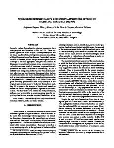
Another valuable aspect of this research can be seen in the kernel formulation which demonstrates warping of the projected patterns towards their respective category axes. This suggests a geometric approach to classification, i.e. we could consider the angle of deviation of a test set pattern from each category axis as a measure of class membership. Within the category space, a base category is represented by the bases (axes) that define the category space. Class membership is therefore inversely proportional to the angle between the pattern and the respective category axis. Figures (1) through (3) illustrate the warped space for various three class problems, for a variation in the width parameter (σ) of a Gaussian radial basis function kernel in the range σ = [0.1, 0.8]. Note the improved visualization semantics of the category space approach when compared to the other dimensionality reduction techniques.

5 Experimental Results

K-CQS

16

K-PCA

K-MC-FLD

Fig. 1: Reduced dimensionality projection for a medium σ value: From top to bottom: Vertebral, Thyroid, Wine, Iris, Seeds.

5 Experimental Results

K-CQS

17

K-PCA

K-MC-FLD

Fig. 2: Reduced dimensionality projection for a small σ value. From top to bottom: Vertebral, Thyroid, Wine, Iris, Seeds.

6 Conclusions

18

K-CQS

K-PCA

K-MC-FLD

Fig. 3: Reduced dimensionality projection for a large σ value. From top to bottom: Vertebral, Thyroid, Wine, Iris, Seeds.

6

Conclusions

In this work, we presented a new approach to supervised dimensionality reduction—one that attempts to learn orthogonal category axes during training. The motivation for this work stems from the observation that the semantics of the multi-class Fisher linear discriminant are unclear especially w.r.t. defining a space for the categories (classes). Beginning with this observation, we designed an objective function comprising sums of quadratic and absolute value functions (aimed at maximizing the inner product between each training set pattern and its class axes) with Stiefel manifold constraints (since the category axes are orthonormal). It turns out that recent work has

6 Conclusions

19

characterized such problems and provided sufficient conditions for the detection of global minima (despite the presence of non-convex constraints). The availability of a straightforward Stiefel manifold optimization algorithm tailored to this problem (which has no step size parameters to estimate) is an attractive by-product of this formulation. The extension to the kernel setting is entirely straightforward. Since the kernel dimensionality reduction approach warps the patterns toward orthogonal category axes, this raises the possibility of using the angle between each pattern and the category axes as a classification measure. We conducted experiments in the kernel setting and demonstrated reasonable performance for the angle-based classifier suggesting a new avenue for future research. Finally, visualization of dimensionality reduction for three classes showcases the category space geometry with clear semantic advantages over principal components and multi-class Fisher. Several opportunities exist for future research. We notice clustering of patterns near the origin of the category space, clearly calling for an origin margin (as in SVM’s). At the same time, we can also remove the orthogonality assumption (in the linear case) while continuing to pursue multi-class discrimination. Finally, extensions to the multi-label case [28] are warranted and suggest interesting opportunities for future work.

References [1] T. W. Anderson and R. Bahadur. Classification into two multivariate normal distributions with different covariance matrices. The Annals of Mathematical Statistics, pages 420–431, 1962. [2] J. Arenas-Garcıa, K. B. Petersen, and L. K. Hansen. Sparse kernel orthonormalized PLS for feature extraction in large data sets. Advances in Neural Information Processing Systems, 19:33–40, 2007. [3] E. Bair, T. Hastie, D. Paul, and R. Tibshirani. Prediction by supervised principal components. Journal of the American Statistical Association, 101(473):119–137, 2012. [4] E. Bair and R. Tibshirani. Semi-supervised methods to predict patient survival from gene expression data. PLoS Biol, 2(4):e108, 2004. [5] P. Belhumeur, J. Hespanha, and D. Kriegman. Eigenfaces vs. Fisherfaces: Recognition using class specific linear projection. IEEE Transactions on Pattern Analysis and Machine Intelligence, 19(7):711–720, 1997. [6] M. Belkin and P. Niyogi. Laplacian eigenmaps for dimensionality reduction and data representation. Neural Computation, 15(6):1373–1396, 2003. [7] C. M. Bishop. Neural Networks For Pattern Recognition. Oxford University Press, 1st edition, 1996. [8] C. M. Bishop. Pattern Recognition and Machine Learning. Springer, New York, 1st edition, 2006. [9] M. Bolla, G. Michaletzky, G. Tusnady, and M. Ziermann. Extrema of sums of heterogeneous quadratic forms. Linear Algebra and Its Applications, 269(1-3):331–365, 1998. [10] R. Duda and P. Hart. Pattern Classification and Scene Analysis. Wiley, New York, NY, 1973.

6 Conclusions

20

[11] R. A. Fisher. The use of multiple measurements in taxonomic problems. Annals of eugenics, 7(2):179–188, 1936. [12] D. H. Foley and J. W. Sammon. An optimal set of discriminant vectors. IEEE Transactions on Computers, 100(3):281–289, 1975. [13] D. R. Hardoon, S. R. Szedmak, and J. R. Shawe-Taylor. Canonical correlation analysis: An overview with application to learning methods. Neural Computation, 16(12):2639–2664, Dec. 2004. [14] T. Hastie and R. Tibshirani. Discriminant analysis by Gaussian mixtures. Journal of the Royal Statistical Society, Series B (Methodological), pages 155–176, 1996. [15] H. Hotelling. Analysis of a complex of statistical variables into principal components. Journal of Educational Psychology, 24(6):417–441, 1933. [16] S. Ji and J. Ye. Linear dimensionality reduction for multi-label classification. In Proc. 21st Intl. Joint Conf. on Artifical Intelligence (IJCAI), volume 9, pages 1077–1082, 2009. [17] R. A. Johnson and D. W. Wichern. Applied Multivariate Statistical Analysis. Pearson, 6th edition, 2002. [18] I. T. Jolliffe. Principal Component Analysis. Springer Series in Statistics. Springer, New York, 2nd edition, 2002. [19] J. Kiefer. Sequential minimax search for a maximum. Proceedings of the American Mathematical Society, 4(3):502–506, 1953. [20] M. Lichman. UCI machine learning repository. http://archive.ics.uci.edu/ml, 2013. [21] C. R. Rao. The use and interpretation of principal component analysis in applied research. Sankhy¯ a: The Indian Journal of Statistics, Series A, 26(4):329–358, 1964. [22] T. Rapcs´ ak. On minimization of sums of heterogeneous quadratic functions on Stiefel manifolds. In From local to global optimization, pages 277–290. Springer, 2001. [23] T. Rapcs´ ak. On minimization on Stiefel manifolds. European Journal of Operational Research, 143(2):365–376, 2002. [24] S. T. Roweis and L. K. Saul. Nonlinear dimensionality reduction by locally linear embedding. Science, 290(5500):2323–2326, 2000. [25] J. W. Sammon. An optimal discriminant plane. IEEE Transactions on Computers, 100(9):826– 829, 1970. [26] B. Sch¨ olkopf and C. J. C. Burges. Advances in kernel methods: Support vector learning. MIT Press, 1999. [27] L. Sun, S. Ji, and J. Ye. Canonical correlation analysis for multilabel classification: A leastsquares formulation, extensions, and analysis. IEEE Transactions on Pattern Analysis and Machine Intelligence, 33(1):194–200, 2011. [28] L. Sun, S. Ji, and J. Ye. Multi-label dimensionality reduction. CRC Press, 2013.

6 Conclusions

21

[29] J. B. Tenenbaum, V. de Silva, and J. C. Langford. A global geometric framework for nonlinear dimensionality reduction. Science, 290(5500):2319–2323, 2000. [30] I. Tsochantaridis, T. Hofmann, T. Joachims, and Y. Altun. Support vector machine learning for interdependent and structured output spaces. In Proc. Twenty-first Intl. Conf. on Machine Learning (ICML), page 104. ACM, 2004. [31] V. Vapnik. Statistical Learning Theory. Wiley Interscience, 1998. [32] D. Widdows. Orthogonal negation in vector spaces for modelling word-meanings and document retrieval. In Proc. 41st Annual Meeting on Association for Computational Linguistics, volume 1, pages 136–143. Association for Computational Linguistics, 2003. [33] D. Widdows. Geometry and Meaning, volume 773. CSLI publications, Stanford, 2004. [34] J. Ye. Least squares linear discriminant analysis. In Proc. 24th Intl. Conf. on Machine Learning (ICML), pages 1087–1093. ACM, 2007. [35] A. L. Yuille and A. Rangarajan. 15(4):915–936, 2003.

The concave-convex procedure.

Neural computation,