A Classification Of Nonlinear Systems: An Entropy Based Approach

A Classification Of Nonlinear Systems: An Entropy Based Approach A. Balestrino, A. Caiti and E. Crisostomi Department of Electrical Systems and Automation, University of Pisa Via Diotisalvi, 2, 56125, Pisa, Italy This paper exploits concepts derived from the thermodynamics of curves for the analysis and classification of dynamic systems. In particular, a new indicator based on an entropy measure is used to retrieve some information about the degree of irregularity of a curve. Irregularity is meant as a distance from the ordered situation of a sequence of points on a straight line. The proposed indicator is used to compare the evolution of trajectories in the state space for any dynamic system, and some of its properties are very interesting for the study and classification of nonlinear systems. Nowadays classification of nonlinear systems is still a tough subject, and there are not yet systematic approaches to tackle it. It would be useful however, especially for industrial applications, to know how much a dynamic system behaves like a linear system. The proposed indicator has interesting properties, in particular it provides a finite value which does not depend on stability issues and it always provides a constant unitary outcome when applied to linear systems. Nonlinearity of a dynamic system can hence be evaluated as a distance from the ideal linear condition. The proposed indicator was then tested for several benchmark problems, also for chaotic systems to emphasize the theoretical expectations.

1. Introduction It might look odd that a powerful concept such the one of entropy, whose importance is extended but not limited to mechanics, thermodynamics, information theory and geostatistics, has not found an essential role in other disciplines, like for instance in the systems theory field. Only a few attempts have been made, see for example (Saridis, 1988) and (Feng et al., 1997), to introduce entropy-based tools in control theory. In this paper an entropy based approach, which is derived from the theory of thermodynamics of curves, like in (Mendès France, 1983), (Dupain et al., 1986) and (Denis and Crémoux, 2002), is suggested and adapted for systems theory applications. A new entropic indicator is introduced with interesting properties. It is different from other known algorithms used to classify nonlinear systems or attracting sets, like Lyapunov exponents, or dimension-like concepts, as in (Parker and Chua, 1987). Classification of nonlinear systems is somehow a tough subject, and there is not yet a systematic approach to tackle it, at least to the authors’ knowledge. Some attempts can be found in (Dragt et al., 1992), where invariant moments of distribution of particles undergoing a Hamiltonian system are investigated, and (Hofstadter and Saridis, 1976), where classification of nonlinear stochastic systems was performed using input-output measurements. In this paper a new indicator is proposed that has the property of

providing a unitary value whenever applied to linear systems. Moreover the proposed indicator does not depend on stability issues and is generally able to describe the disorder or irregularity in the evolution of a dynamic system. By irregularity it is meant a distance from an ordered sequence of points along a line. The proposed indicator can be used within any dynamic system; differences arise when the steady state is an equilibrium point, or the attracting set is a periodic sequence or presents a chaotic behaviour. The paper is organized as follows: next section is dedicated to a review of the entropy of curves and basic concepts from thermodynamics of curves are recalled. Section 2 shows how the entropy indicator has been developed within a system theory framework and the most important properties of the proposed algorithm are proved. In the third section examples are shown from nonlinear benchmark problems, both presenting periodic and chaotic behaviours. In the last section some conclusions are given, and some future work is outlined.

2. Thermodynamics Of Curves Notions about thermodynamics of plane curves can be found in (Mendès France, 1983) and (Dupain et al., 1986); here the fundamental concepts are reviewed using the same notation as in (Denis and Crémoux, 2002) to provide the most important mathematical basis for the proposed approach. The starting point is a finite curve Γ of length L. Let Cr be the convex hull of Γ and C the length of its boundary. From a theorem of Steinhaus, the expected value of the number of intersection points of a random line D with a plane curve is computed as in equation (1): E[D ] =

∞

∑ nP

n

=

n =1

2L C

(1)

where P is the probability for a line set to intersect a plane curve in n points. n Probability is computed as the number of lines which intersect the plane curve with respect to the total number of intersecting lines. If we consider now a probability distribution p = ( p1 , p 2 ,..., p n ) , such that pi ≥ 0 for all I, and n

∑p

i

=1

(2)

i =1

Shannon’s measure of entropy (or uncertainty) for such a distribution is given by equation (3): S n (p ) = −

n

∑ p log(p ) i

i =1

i

(3)

By analogy the entropy of a curve Γ can be defined as (Mendès France, 1983) H(Γ ) = −

∞

∑ P log(P n

n

)

(4)

n =1

If we consider all the probability measures which satisfy Steinhaus theorem, and maximise entropy using Gibb’s equilibrium measure, then the maximal entropy is Pn = e

− βn ⎛ β ⎞ ⎜ e − 1⎟ ⎝ ⎠

(5)

where ⎛ 2L ⎞ β = log⎜ ⎟ ⎝ 2L − C ⎠

(6)

Combining then equations (4), (5) and (6), we find the function of entropy of a plane curve Γ, (Mendès France, 1983) β ⎛ 2L ⎞ H (Γ ) = log⎜ ⎟+ ⎝ C ⎠ eβ − 1

(7)

The entropy function of a plane curve is characterized by the length L of the line and the length C of the complex hull. In literature, thermodynamics of curves has been applied to the study of time series, where the length L is the measurement of the fluctuating tortuous path of a curve in a plane, while C is assumed to be a time (Denis and Crémoux, 2002). In the next section it is shown how the entropy of a curve can be rearranged in a different context to suggest a classification of nonlinear systems.

3. Application Of Entropy Of Curves To State Space Analysis Of Dynamic Systems This section shows how theoretical concepts from thermodynamics of curves have been exploited to propose a classification of nonlinear systems and provides some properties of the proposed approach. Supposing to start from a discrete state-space formulation of a dynamic system, x (k + 1) = f (x (k ), Ts )

x ∈ ℜn

(8)

External inputs can be included in the previous equations without significant changes, and have not been considered here just for sake of simplicity. The general idea is to consider a cloud of particles, which represent points in the state space, and to study how the cloud of points evolves in time. If we consider the line that joins all the points together, it is possible to study how the entropy of the curve changes with time,

according to equation (9), which is an extension to more dimensions of equation (8), more suitable for systems theory applications. Following the approach of (Denis and Crémoux, 2002), we obtain ⎛ 2L ⎞ H(Γ ) = log⎜ ⎟ ⎝ d ⎠

(9)

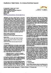
where the logarithm is referred to base 2. Therefore, as can be seen from equation (9), computation of the convex hull in ℜ n was substituted by computation of the diameter d of the smallest ball that encloses all the particles. Definition of the entropy indicator as in equation (9) has an intuitive meaning: a straight line has a unitary entropy, while entropy increases with the irregularity of the curve as shown in the figure below. H=1

H = 1 13

H = 2 14

The figure shows the different entropy values for different lines that have the same endpoints. The entropy indicator clearly depends on the irregularity of the curve

Hence computation of the entropy of a curve is performed by choosing a prespecified number of particles along a straight line and making them evolve independently. The entropy indicator has special properties that are listed below. Their proofs can be found in (Balestrino et al., 2007). Remark 1: H(k) as defined in equation (9) is always a finite number. Remark 2: H(k) as defined in equation (9) depends on the logarithm of the number of particles. Remark 3: A cloud of particles ordered sequentially along a straight line has a constant value of H(k), as defined in equation (9), equal to 1. Lemma: H(k) as defined in equation (9) has a constant value 1 when applied to linear systems.

4. Examples of the Proposed Indicator In the previous section it was shown that the proposed indicator provides a constant unitary value when applied to linear systems, thus suggesting that it could be used for nonlinear systems to verify how much a nonlinear system is far from the ideal linear condition. This would be a very useful notion for many industrial applications in several

fields. In this section many benchmark problems have been studied from the entropy of curves point of view, looking for common patterns.

H(k) in Kaprekar dynamic system

H(k) in Lorentz dynamic system

H(k) in Van Der Pol system

H(k) in a logistic chaotic system

H(k) in a logistic non chaotic system

H(k) in a linear dynamic system

The previous figures represent evolutions of the proposed indicator for different dynamic systems. From left to right and from top to down they represent Kaprekar, see for example (Salwi, 1997), Lorentz, Van der Pol, logistic with chaotic behaviour, logistic without chaotic behaviour and linear equations. As can be seen, the first four

figures are rather similar, although they represent chaotic systems (Lorenz and logistic equations) and dynamic systems with a periodic limit cycle (Van der Pol and Kaprekar equations). The same logistic example behaves differently according to the chaotic parameter, as is evident from a comparison between the fourth and the fifth figure. The linear example provides finally a constant unitary value. Classification among the nonlinear systems can rely on the steady state value of the entropy indicator, whose module clearly separates linear or quasi-linear behaviours from periodic and completely nonlinear behaviours. Also rise times and solution times provide some more information about the overall nonlinearity of the dynamic system.

4. Conclusions The paper proposes a classification of nonlinear systems based upon an entropy of curve approach. The mathematical basis and the analytical properties are thoroughly provided, together with a series of examples that shows the behaviour of the proposed algorithm. The entropy indicator is hence able to distinguish linear from nonlinear systems, and to classify nonlinear systems through a degree of nonlinearity. Some ongoing work is now been developed to find some more properties of the proposed indicator and to find whether the irregularity of each nonlinear system can be used to provide some more insight about dynamic systems. A valid framework to tackle a classification of nonlinear systems would be very useful for process control applications in different fields, to predict the behaviour of the dynamic system.

6. References Balestrino, A., A. Caiti and E. Crisostomi, 2007, Entropy of curves for nonlinear systems classification, submitted to IFAC Symposium on Nonlinear Control Systems. Denis, A. and F. Crémoux, 2002, Using the entropy of curves to segment a time or spatial series, Mathematical Geology 34, 899-914. Dragt, A., F. Neri and G. Rangarajan, 1992, General moment invariants for linear Hamiltonian systems, Phys. Rev. A 45, 2572-2585. Dupain, Y., T. Kamae and M. Mendès France, 1986, Can one measure the temperature of a curve, Arch. Rational Mech. Anal. 94, 155-163 Feng, X., K.A. Loparo and Y. Fang, 1997, Optimal state estimation for stochastic systems: an informatic theoretic approach. IEEE transaction on Automatic Control 42, 771-785 Hofstadter, R. and G.N. Saridis, 1976, Feature selection for onlinear stochastic system classification. IEEE trans. on Aut. Control 21, 375-378 Mendès France, M., 1983, Les courbes chaotiques, Courrier du Centre National de la Recerche Scientifique 51, 5-9 Parker, T.S. and L.O. Chua, 1987, Chaos: a tutorial for engineers. Proc. IEEE 75, 9821008 Salwi, D., 1997, Scientists of India, CBT Publications Saridis, G.N., 1988, Entropy formulation of optimal and adaptive control, IEEE trans. on Aut. Control 33, 713-721.