A General Mining Method for Incremental Updation in Large Databases*t ShieJue Lee Department of Electrical Engineering, National Sun Yat-Sen University, Taiwan
[email protected] .edu .tw
Wan-Jui Lee Department of Electrical Engineering, National Sun Yat-Sen University, Taiwan
[email protected] Abstract - The database used for knowledge discove y is dynamic in nature. Data may be updated and new transactiom may be added ouer time. As a msult, the knowledge discovered from such databases is also dynamic. Incremental mining techniques have been developed to speed up the knowledge discovery PTOcess by avoiding re-learning of rules from the old data. To maintain the large itemsets against the updated database, we develop an approach named Negative BOTder using Sliding- Window Filtering (NB-SWF) which adopts the idea of the negative border and the slidingwindow filtering algorithm. Negative border can help reduce the number of scans over the original database and the sliding-window filtering algorithm is to discover new itemsets in the updated database. By integrating the sliding-window filtering algorithm with the negative border, a lot of effort in the re-computation of negative border can be saved, and the minimal candidate set of large itemsets and negative border in the updated database can be obtained eficiently. Simulation results have shown that the NB-SWF runs faster than other incremental mining techniques, especially when there are few new large itemsets in the updated database.
Keywords: Incremental mining, association rules, temporal mining.
1
Introduction
So far, there are three directions of incremental mining, i.e., apriori-based, negative border, and slidingwindow filtering(SWF). Apriori-based algorithms, e.g. FUP2 [3], level-wisely update the existing large itemsets when transactions are added to or deleted from the database and tend to suffer from the problem of multiple scans of database. The negative border [6] consists of all itemsets that were candidates but did not have enough support while computing large itemsets in the original database and is used to compute the new set ‘Supported by the National Science Council under the grants NSC-91-2213-E110-024 and NSC-91-2213-E-110025. t0-7803-7952-7/03/¶17.00 @ 2003 IEEE.
of large itemsets in the updated database in [6]. The availability of the negative border of the set of large itemsets and their counts in the original database can reduce the number of scans over the database to at most once [4, 71. However, the recompution of negative border deteriorates the performance of this method. Sliding window filtering (SWF) [ 5 , 21, on the other hand, segments the database into several partitions and employs the minimum support threshold in each partition to filter unnecessary candidate 2-itemsets. Under SWF, the cumulative information of mining previous partitions is selectively carried over toward the generation of candidate itemsets for the subsequent partitions. In SWF, one scan over the updated database is necessary to find out the large itemsets from the candidate ones. In this paper, we develop an approach named NBSWF, which integrates the SWF algorithm with the negative border to save a lot of effort in the re-computation of negative border and obtains the minimal candidate set of large itemsets and negative border in the u p dated database efficiently. Moreover, unnecessary scans over the database can be omitted in NB-SWF. In other words, we compute a small set of candidate itemsets in an efficient way, and the scan over the database with the candidate itemsets can be saved if not necessary. The rest of the paper is organized as follows. In Section 2, we briefly describe the concept and application of negative border. In Section 3, the technique of SWF is introduced. In Section 4, we describe our method, NB-SWF, in detail. We give an example to illustrate the NB-SWF in Section 5 . Simulation results are p r o sented in Section 6, and finally, a conclusion is given in Section 7.
2
Negative Border
As mentioned earlier, in (61, the concept of negative border is used to compute the new set of large itemsets in the updated database. The negative border consists of all itemsets that were candidates but did not have enough support while computing large itemsets in the original database, DB. That is,
1423
NBD(Lk) = Ck - Lk,
(1)
Table 2: Candidate Z-itemsets generated after scanning partition PI. I P. I
Table 1: An illustrative transaction database. Partition I TID I Items I I I 1 I A.C.D.E.F 1
AD AE
1
2
1
2
-
Table 3: Candidate 2-itemsets generated after scanning .ition Pz and P3, respectively. I/
D-
where CI,is the set of candidate k-itemsets generated by Lk-1; LI, is the set of large k-itemsets and, N B D ( L I , ) is the set of k-itemsets in the negative border of the set of large itemsets L. In other words, the negative border contains the closest itemsets that could be frequent. For example, let R be a set of items = A, B , ...,F and assume the collection of S of large itemsets is { A } , { B } , IC), IF), { A , B } , { AC ) , { A ,F } , IC, F ) , { A ,C,PI. Then, the negative border for the above collection is N B D ( S ) = { { D ) , { E } , { B ,C),{ B ,F ) } .
3
AB
I
count __ ~
2
3
.2
6 5 5 4
1 1 2
AF
2
EF
4 6 3
1 1
DE DF
2 2 ~ ~
__ ~
Sliding-Window Filtering
SWF [5] is an incremental mining algorithm that divides the database into partitions and sequentially p r e cesses the partitions one by one. In th processing of a partition, a progressive set of candidate 2-itemsets, CZ, is generated. The concept of the algorithm is described as follows. Suppose the database is divided into n partitions PI&, ...,P,,, and the partitions are processed one by one. For each large itemset I, there must exist some partition Pk such that I is large from partition Pk to Pn. If we know a candidate 2-itemset is not large from the starting partition where it becomes large to current partition PI,,this itemset can be deleted. If this itemset is indeed large, it must be large in some partition PI,,, where k' > k, and we can add it to CZ again. Thus, for each partition P,, SWF adds new partial large 2itemsets of P, into CZ , records its starting partition P, and counts, and checks if the present itemsets in CZ are continually large from its starting partition to partition P,. If a candidate 2-itemset is no longer partially large, this itemset is removed from C z . After all partitions have been processed, the candidate 2-itemsets, CZ, which is close to the large 2-itemsets, will be obtained. For the moderate number of candidate %itemsets, all candidate k-itemsets, where k >= 3, can be generated from candidate 2-itemsets. Finally, one database scan is applied to calculate the supports of all candidate itemsets and determine the large ones In the following, we use an example to illustrate the algorithm of SWF. Suppose we have 9 transactions in the database, as shown in
Table 1, and the database is segmented into three partitions, P I , Pz, and P3. The minimum support threshold is set to 0.4. To generate CZ, we scan each partition sequentially. After scanning the first segment of 3 transactions, candidate 2-itemsets AD, AE, DE, D F are generated with two attributes start partition PI and count as shown in Table 2. Similarly, after scanning partition Pz, the counts of potential candidate 2-itemsets are recorded in Table 3. Note that the filtering threshold of those itemsets carried over from the previous phase is [(3+3) x 0.4]=3 and that of newly identified candidate itemsets is r3 x 0.41 =2. It can be seen from Table 3 that we have 9 candidate itemsets after processing partition P z , and 4 of them are carried over from the partition PI and 5 of them are newly identiied in partition Pz. Finally, the resulting candidate 2-itemsets after processing P3 are AB, AD, AE, AF, BF, D E , DF, EF as shown in Table 3. Note that though appearing in the previous phase Pz,itemset B E is removed from C2 once P3 is taken into account since its count does not meet the filtering threshold then, i.e., 2 < 3. Consequently, we have 8 candidate 2-itemsets generated by SWF. Note that 7 of those 8 candidate 2-itemsets are large Z-itemsets which shows that CZis close to Lz.
4
1424
Negative Border using SlidingWindow Filtering (NB-SWF)
For easy exposition, the meaning of symbols used are given in Table 4. The problem of incremental mining
Proof: By Eq.(l), we have Cz = Lz U N B D ( L 2 ) . Obviously, Lk G C k , and therefore apriori-gen(L&apriori-gen(Ck), where &+I UNBD(Lk+l)=apriori-gen(Lk) and Ck+l=apriori-gen(Ck), for k >= 2. That is, L ~ +UI NBD(Lk+l) C Ckfl for k >= 2, Therefore, L U N B D ( L ) C C is derived, and the assumption that V I E L U N B D ( L ) , I E C is proved.
Table 4: Meaning of symbols used. svmbol I meanine DB I the original database number of transactions in database d the set of newly added transactions the set of deleted transactions the updated database ( D B - A- + A+) partition P, to P3 in database D B number of transactions in db”) containing itemset I minimum support threshold number of transactions in partition Pk number of transactions in partition P, containing itemset I large itemsets of t h e original database candidate itemsets of the original database L’ large itemsets of the updated database C‘ candidate itemsets of the updated database ~
is to find the set of large itemsets L’ in the updated database DB‘. L’ may contain some new itemsets called emerged itemsets. Some itemsets from L , called declined itemsets, may be absent in L’. Those itemsets which exist both in L’ and L are retained itemsets.
4.1
Description of the Algorithm
In order to solve the incremental mining problem effectively, we maintain the large itemsets and the negative border along with their support counts in the database. That is, for every I E L U N B D ( L ) , we maintain t D B ( I ) . However, the number of 2-itemsets in L U N B D ( L ) is usually too big and therefore costs memory and reduces computational efficiency. Thus, we adopt the SWF to filter unnecessary 2-itemsets in NBD(L2). That is, the C, in Eq.(l) is the set of candidate 2-itemsets, C,, generated by SWF instead of L1. Since Cz is close to L2 as shown in Section 3, our set of N B D ( L 2 ) is much smaller than that in [SI. In the first step of our algorithm, we use SWF to compute candidate itemsets as introduced in Section 3. Then, one database scan is applied to calculate the s u p ports of all candidate itemsets and the large ones and the negative border can further be determined by t h e orem 1 . Secondly, to maintain the itemsets through data addition and deletion, we count the support in A+ and A- for all itemsets in L U N B D ( L ) . If an itemset I E L does not have minimum support in DB’, then I is removed from L. This can be easily checked since we know the support count for I in D B , A+ and A-, respectively.
On the other hand, there could be some new itemsets which become large in the updated database. Let I be an itemset which becomes a large itemset of the u p dated database. We know that some subset of I should be moved from N B D ( L ) to L‘ [6, 71. If it is not, some 2-item subset of I must be the newly identified candidate 2-itemset in the updated database. Thus, if none of the itemsets in N B D ( L ) gets minimum support and no newly identified candidate 2-itemsets are generated in the updated database, no new itemsets will be added to L’ and there is no need to scan the updated database for discovering new large itemsets. However, if some itemsets in N B D ( L )get minimum support or the count of some newly identified candidate 2-itemset in A+ is larger than 1s t I A+ 11, the candidate itemsets are recomputed. As shown in theorem 2, a newly identified candidate 2-itemset will not be an emerged itemset, if it is not large in At. Thus, the threshold rs*lA+ll is used to reduce the influence of the unqualified itemsets and save the unnecessary scans over the database. For those newly identified itemsets in the candidate itemsets, one database scan is applied to calculate the supports of them and determine the large ones and the negative border. Theorem 2: If I is a newly identified candidate 2-itemset in A+ and it is large in DB’, the count of I in A+ must be greater than 1s t I A+ 11.
Proof: Since I is a newly identified candidate 2-itemset in C;, it is not in the set of candidate 2-itemsets Cz of DB. Moreover, the candidate 2-itemsets of ( D B - A-) are generated by removing unqualified itemsets from CZ,thus I is also not a candidate 2-itemset of ( D B - A-). That is, I will not be a large itemset in(DB - A-). Assume that I is also small in A+. I must be small in ( D B - A-) + A + , which is DB’. This results in a contradiction. Thus, the assumption that I is small in A+ is not correct Theorem 1: For all itemset I , where I is in L U N B D ( L ) , and I must be large in A+. 1 must also be in the candidate itemset C.
1425
4.2
Pseudo-Code for the Program
Table 5: A set of newly added transactions. I Partition I TID I Items I
i ]
Our algorithm is presented in a high-level description of program code as follows. Note that the set of candidate 2-itemsets, CZ, used in functions negativehorderpen() and Update-Large-Itemset() is initially generated by the function preprocessing() given in [ 5 ] , and the function apriori-gen() which is called by Update-LargeItemset() can be found in [I,7, 41.
AGF
A,C
function negativeborder-gen(Cz,L) Split L into Lz, ...: L,, where n is the size of the largest itemset in L ; for all k = 2, ..., n do compute Ck+i using apriori-gen(Lk); L U ~ B D ( L ) = U k = ~ , . . . , , +C lk ; end negativeborder-gen
L'=L'
uz;
L'=L' zf (L' is not C L ) or (31, where I E Ci, I Cz and t a + ( I )2 1s * I A+ 11) then h = 2; whzle (CL # @ ) d o compute using apriori-gen(Ci); h=h+l: New-Candidate= C' - ( L U N B D ( L ) ) ; zf (New-Candidate# 0 ) then for each itemset I E New-Candidate do af ( t D s , ( ! ) 2 1s * IDB'I1) then
c;+~
-
function Update-Large-Itemset(L,NBD(L),Cz) DB=C;=,, p k ;
A-=C'-lk=m p k l
A+=C3k=n+l p k ; DB'=DB - A-
c; = cz;
//one scan of
+ A'=C;=,,
Pk;
A-
L'=L ul; . .
for k = m to (i - 1) do
for each itemset I E L U N B D ( L ) do t ( D B - a ~ ) ( l ) = t ( D B - n - ) (z )tPk (1); (Initially, t(DB-&)(I)=tDB(I).) for each 2-itemset I E Pk do if I E c; and I.staTt I k I.count = I.count - t p , ( I ) ; 1.start = k + 1:
//one scan of A+ for k = ( n 1 ) to j do for each itemset I E L U N B D ( L ) do
+
.ijI$c; I.count = t p , ( I ) ; Istart = k; if (1.count 2 1s * IPkll)
N B D ( L ' )=negativeborder-gen(C;,L'); end Update-Large-Itemset
5
. .
tDB'(I)=tDB'(I)+ t P k ( i ) ; (Initially, t o B , ( I ) = t ( o B - n ~ ) ( I ) . ) for each 2-itemset I E P k do if I E C; 1.cmnt = I.count t p , ( I ) ; if (I.count < Ts * Cz"=l..t.7t(lPzl)l) c; = c; - I ;
+
UI :
for each itemset 1 E N B D ( L ) do Zf ( t D B ' ( 1 ) 2 [S * IDB'I1) then
An Example
We give an example to illustrate the NB-SWF in this section. Use the database given in Table 1 as the original transaction database, and the first partition PI is extracted as the set of deleted transactions, A-. Snppose we have a set of newly added 6 transactions, A+, as shown in Table 5. Note that lDBl = 9, [A' I = 6, [ A- I = 3, and IDB'I = 12. The minimum support threshold is set t o 0.4. Thus, a n itemset I must he present in at least 5 transactions in DB' in order t o be a large itemset in L'. The execution of the algorithm is described below. Initially, CZ is derived as shown in Section 3. After the candidate set Cis generated by Cz, one scan over the database D B is given t o determine L and N B D ( L ) . For D B , the sets of large k-itemsets, Lk, and their negative borders, N B D ( L k ) , where k >= 2, along with their counts are as follows:
Lz =
c;=c;ul;
{ ( A D , 6 ) ,( A E , 5 ) ,(AF-61,( B F , 5 ) ,
.
L'=0;
I.
~
.
(2)
for each itemset I E L do i f ( t D B , ( I ) 2 [s * IDB'I1) then
Then, the updated portions of the database are scanned 1426
Table 6 Candidate 2-itemsets, Ci, generated after deleting partition A- and then adding partition A+. I -AII CA+ I .~ II itemset 1 start I count 11 itemset I start I count ~
CF
AF BF
2
4
DF
2
4
DF
2
5
in order to find the candidate 2-itemsets, Ci, in the u p dated database, as shown in Table 6. In the scan of Aand A+, the support counts of itemsets in L U N B D ( L ) are also maintained. Thus, L and N B D ( L ) , along with their supports after scanning A- and A+, are: Lz =
6.1
L; = { ( A F ,71, (BF,6),(DF,5)}, NBD(L;) = { ( E D ,4),(CF,4)).
Experiment 1
Five datasets mentioned above are used to conduct several experiments to evaluate the relative performance of NB-SWF and SWF. In Figure 1, we average the ex-
,”*
{ ( A D ,41%(AE,’3),( A E 7),( B F ,61,
Next, for each itemset in L , if its support count in DB‘ is larger than 5, it will be included in L‘. Therefore, A F , B F , and DF are now included in L’. These itemsets are so called retained itemsets. Moreover, we have to find out those emerged itemsets. In this step, the negative border and Ck are firstly used to discover whether there are emerged itemsets. Though there is no itemset moved from negative border to L‘, but the count of the newly identified candidate 2-itemset, C F , in A+ is equal to [s*(lA+1)1=3. So, there may be some emerged itemsets in the updated database, and the candidate itemsets are recomputed. Finally, one database scan over DB‘ is applied to calculate the supports of new candidate itemsets, B D and CF. Therefore, the final set of large itemsets and negative border in DB’ are:
6
... ,and T10.14.DlOOK.C50%,are used in the experiments where T is the mean size of a transaction, I is the mean size of potential maximal large itemsets, D is the number of transactions in units of K, i.e., 1000, and C is the correlation between items in terms of percentage. In the following, we give three different experiments to compare the performance of the incremental mining methods mentioned above on different scales of incremental portion, support threshold and correlation between items, respectively. Experiments results demonstrate our NB-SWF performs better than other incremental mining methods under all kinds of situations.
(4)
Experimental Results
We compare the performance of our NB-SWF with that of SWF [5]by running them on several experiments with a PC with AhlD Athlon XP CPU and 1.OG memory. In the experiments, we use synthetic data to form input databases to the algorithms. The database of size IDB+A+l is generated using the same technique as introduced in [l], and the first lDBl transactions are used as D B and the next I A+ I transactions as A+. The first I A- 1 transactions of D B are used as A-. Five datasets, T10:14.DlOOK.C10%, T10.14.DlOOK.C20%,
,
,
.
.
,
.
,
,
,
,
Figure 1: Performance comparison between NB-SWF and SWF. ecution time of NB-SWF and SWF in 5 datasets and 4 fractional sizes for each support threshold. It can be seen that NB-SWF outperforms SWF with all support thresholds. With low support thresholds, large number of candidate itemsets are generated, but only few of them are scanned over the updated database in NBSWF. With medium or high support thresholds, NBSWF may not have to scan over the updated database since no emerged itemsets are found.
6.2
Experiment 2
In this experiment, we use different fractional sizes, i.e., 1%, 2%, 5% and lo%, of the dataset T10.14.DlOOK.C30% as the size of the deletion and addition datasets, respectively. In Figure 2, we show the speedup ratio S R of NB-SWF over SWF for fractional sizes 1%, 2%, 5% and lo%, respectively. The speedup ratio S R is calculated as follows:
1427
SR =
time for SWF - time for NB-SWF time for NB-SWF
(5)
~
of larger incremental sizes, correlations, and thresholds.
7
Figure 2: The speedup ratios of NB-SWF over SWF for fractional sizes of 1%, 270, 5% and 10% with dataset T10.14.DlOOK.C30%.
Conclusion
In order to solve the incremental mining problem effectively, we develop an approach named Negative Border using Sliding-Window Filetering (NB-SWF) which adopts the idea of the negative border and the sildingwindow filtering algorithm. The negative border is used to avoid unnecessary scans over the updated database. The candidate set is generated in one shot with SWF, and thus we need a t most one scan over the updated database. Since the number of scans over the updated database is greatly reduced, NB-SWF is quite suitable for very large databases. In summary, our incremental mining method is effective and efficient for knowledge updation in large databases.
References [l] R. Agrawal and R. Srikant,“Fast Algorithms for Mining Association Rules,” In Proceedings of the International Very Large Database Conference , pp. 487-499, 1994.
[2] C.H. Chang and S.H. Yang, “Enhancing SWF for Incremental Association Mining by Itemset Maintenance,” In Proceedings of the seventh PacificAsia Conference o n Knowledge Discovery and Data Mining, pp. 301-312,2003.
Figure 3: Performance comparison between NB-SWF and SWF for datasets with correlations of lo%, 20%, 30% and 40%, respectively. Figure 2 shows the speedup ratios for all cases. Apparently, NB-SWF rnns faster than SWF. For larger fractional sizes or larger support thresholds, our speedup is higher since a larger A+ will have a larger possibility to be a good sample of the original and the probability of recomputing candidate itemsets is smaller.
6.3
Experiment 3
We use four datasets having different correlations between items with the fractional size being 5%. The speedup ratios of NB-SWF over SWF are shown in Figure 3 for these four datasets. When the correlation between items in the dataset is weaker, there is a larger chance to discover new large itemsets in all support thresholds. Thus NB-SWF performs much better than SWF in datasets with higher correlations between items. In summary, NB-SWF performs better than SWF for all types of incremental databases, especially in the case 1428
[3] D.W. Cheung, S.D. Lee and B.Kao, ‘‘ A General Incremental Technique for Maintaining Discovered Association Rules,” In Proceedings of the 5th h t e r national Conference o n Database Systems for Advanced Applications, pp. 185-194, 1997.
[4] W.J. Lee and S.J. Lee, “An Efficient Mining Method for Incremental Updation in Large Databases,” to appear in Proceedings of the 4th International Conference on Intelligent Data Engineering and Automated Learning, 2003.
[SI C.H. Lee, C.R. Lin and M.S. Chen, ’‘ SlidingWindow Filtering: An Efficient Algorithm for Incremental Mining,” In Proceedings of the AGM 10th International Confeznce onlnfonnation and Knowledge Management, pp. 263-270, 2001.
[6] S. Tomas, S. Bodagala, K. Alsabti, and S. Ranka, “An Efficient Algorithm for the Incremental U p dation of Association rules in Large Databases,” In Proceedings of the International Conference on Knowledge Discovery and Data Mining , pp. 263266, 1997. [7] N.L. Sarda and N.V. Srinivas, “An Adaptive Algorithm for Incremental Mining of Association Rules,” In Proceedings of DEXA Workshop , pp. 240-245, 1998.