Author manuscript, published in "Third International IEEE Conference on Signal-Image Technologies and Internet-Based System, SITIS'07, Shanghai : China (2007)" DOI : 10.1109/SITIS.2007.25
A colour correlation-based stereo matching based on 1D windows S´ebastien Lefebvre, S´ebastien Ambellouis INRETS-LEOST, 20, rue Elis´ee Reclus 59666 Villeneuve d’Ascq, FRANCE
hal-00521116, version 1 - 25 Sep 2010
{sebastien.lefebvre, sebastien.ambellouis}@inrets.fr
Abstract— In this paper, we propose an original approach to colour correlation-based stereo matching with mono-dimensional windows. The result of the algorithm is a quasi-dense disparity map associated with its confidence map. For each pixel, correlation indices are computed for several widths of windows and several positions of the current pixel. Three criteria, extracted from each correlation curve, are combined by a fuzzy filter to define a confidence measure. A basic decision rule computes the disparity value and its associated confidence for the most of the image pixels. A first study shows results obtained on grey level images with our 1D method and a classical 2D method. Here, the 1D approach presents better results. Moreover, our method is applied to the RGB colour space. A disparity map is computed with each of the three colour components. A fusion step allows to compute the disparity values based on these three disparity maps. The method is validated on the Tsukuba image pair. In the first time, we show that our method presents lower error rates with the RGB colour space than with the grey level image and this, for identical density rates. In a second time, our results (with the colour way) are compared in terms of errors and density rate with those obtained using similar colour 2D methods (presented on the Middlebury website). Our algorithm is ranked in the first places for each area of the image.
I. INTRODUCTION A. Window-based stereo matching Stereovision is a typical problem in computer vision and in 3D reconstruction. Given two images — called left and right images — capturing a scene at the same time from two points of view, stereo techniques aim at defining conjugate pairs of pixels, one in each image, that correspond to the same spatial point in the scene. The difference between positions of conjugate pixels, called the disparity, yields the depth of the point in the 3D scene. Sparse or dense disparity maps can be computed. Sparse disparity maps are produced by stereovision algorithms matching features like edges or corners. Dense disparity maps are computed by algorithms based on the analysis of the grey levels or colours of pixels in a neighbourhood centred on each pixel of the images. In both cases, because of the epipolar geometry, the conjugate of a pixel in the first image lies on the corresponding epipolar line in the second image. This allows one to restrict the matching process to epipolar lines. In the following sections, we focus our attention on dense stereo approaches based on the analysis of a pixel neighbourhood. In these methods, the pairs of conjugate
Franc¸ois Cabestaing LAGIS - UMR CNRS 8146 Bˆatiment P2 - USTL, Cit´e Scientifique 59655 Villeneuve d’Ascq, FRANCE
[email protected]
pixels are computed by maximising (or minimising) a similarity (dissimilarity) function. The properties of this function depend on the grey level or colour distributions in the two windows centred on pixels of epipolar lines. On the one hand, the selection of window shape and size is crucial for the success of matching. The dense stereo algorithms assume that all pixels within the windows have the same disparity. Therefore, the windows must not be too large. On the other hand, if the window is too small, the data available to estimate the similarity function are not sufficient. In literature, several window-based approaches have been presented to deal with this trade-off. Kanade and Okutomi have proposed an adaptive neighbourhood method [1], in which they iteratively modify the neighbourhood size and shape according to the local variation of the intensity and current depth estimates. P´erez et al. also use a neighbourhood with variable shape determined by analysing the similarity between pixels [2]. Some authors use shiftable windows methods: Fusiello et al. have presented a Symmetric Multi-Window (SMW) algorithm [3]. They compute the SSD (Sum of Squared Differences) on nine rectangular windows in which the current pixel is positioned at different places, and keep the window with the smaller SSD. Hirschm¨uller combines the correlation computed on the window centred on the considered pixel with the correlations computed on several support windows [4]. In these algorithms, the modification of window configuration is based on one or several parameters defining the confidence granted to the matching. This notion is essential in some applications, especially for multisensor fusion algorithm and several confidence measures have been described in literature [5]. In [4], the author analyses the relative difference between the two lowest minima of the correlation function. If this value is higher than a fixed threshold, the window configuration is validated and the confidence is high. In [6], the matching is marked as good if the global minimum of the correlation function is sharp. If the confidence is low, several authors prefer to mark the pixels as unmatched and provide semi-dense disparity maps. B. 1D vs 2D correlation window All the previously cited authors describe methods assuming that the images have been rectified [7]. In this case, the conjugate pairs of pixels are located on a single and
hal-00521116, version 1 - 25 Sep 2010
same line in the left and right image. Usually, authors compute correlation indices with two-dimensional windows shifted along the raster lines to deal with textureless area and increase the density of the disparity map. Unfortunately, when neighbour pixels within the window do not have the same disparity, errors appear. In images of real scenes, this fronto-parallel plane assumption — i.e. assumption that all the pixels have the same disparity — is regularly violated because of the perspective effect or because complex objects cannot be accurately described with planes. In this case, disparity errors and a blurring effect across depth discontinuities appear in the resulting map. Moreover, the larger the size of the 2D window, the higher the error rate. In our work, we assume that the information located on the epipolar line, e.g. the single raster line, is sufficient to provide a good matching. In the following sections, we will present an original stereo algorithm using 1D correlation windows and a fuzzy logic filter. Each pixel is labeled with a disparity and the associated confidence value. A basic decision step determines the disparity value and its confidence for the most of image pixels. Indeed, in the case of occlusions or in untextured areas, no information is locally available and most area-based methods compute wrong disparities. To minimize the effect of this drawback, we propose a quasidense method. C. Colour correlation-based matching In computer vision application, the choice of colour space is important. However, a lot of colour spaces have been proposed; In [8], Vandenbroucke et al. have classified the most of the used colour spaces. Several authors have used colour information for correlation-based stereo matching algorithm. Indeed, as presented in [9], the use of colour images can improve the accuracy of stereo matching. The authors have tested their stereo matching method with nine different colour spaces: The results show that colour always improves matching however the best colour space is not easy to underline. In this paper, we aim at taking into account the colour information with our 1D grey level matching approach. We compute a disparity map with each colour component and combine the results in order to have a denser and more precise disparity map. The paper is organised as follows. In Section 2, our 1D windows-based approach is described. Section 3 presents the first results obtained on grey level image; A comparison is done with results computed with the classical 2D method of Hirschm¨uller using the Middlebury evaluation framework. In Section 4, we introduce the use of colour information by detailing the combination method. The colour way is compared to the grey level one. So, our disparity map is compared to maps computed by four other similar colour methods related in literature. The last Section is dedicated to conclusions and outlines future studies.
II. THE 1D APPROACH The proposed method relies on a particular combination of correlation scores computed on several 1D windows. It provides a disparity map associated to a confidence map. The confidence map indicates the level of certainty of each matching, which can be low for example in untextured regions. The overall method is composed of the four steps presented in figure 1. The following sections describe each step, except the left and right consistency (LRC). LRC is a very classical method used to remove incorrect matchings that has already been widely presented in the literature. The reader can find a detailed explanation of this technique in [5]. In the figure 1, the correlation scores, the confidence values and the final disparity map can be computed using various tools and theories. In this part, we present a case study in which the most basic techniques are used for each stage. Two epipolar rectified images ? 1. Calculate similarity measures in each pixel via 1D window-based method (several widths - several positions) ? 2. Model confidence value for each similarity measure ? 3. Decision-making process Select the most confident disparities ? 4. Left-Right Consistency Remove some of incorrect matches ? Final disparity and confidence maps
Fig. 1.
Algorithm outlines.
A. Similarity measure Classical area-based dense stereo algorithms assume that all pixels within correlation windows have the same disparity. Determining the optimal correlation window is crucial for the success of matching, but doing this a priori without specific knowledge about the scene is often impossible. Selecting a specific window size and shape corresponds to making a decision at the beginning of the process. We propose to postpone the decision until the last stage of the matching process. Thus, we compute 1D correlation scores for several widths of the window and several positions of the current pixel. Let wn = 2n+1 be the width of a 1D window Ωn , where n is an integer in the range [1, nmax ]. The window corresponds
to a neighbourhood of the reference pixel (x, y). Let pi be the position of the reference pixel in Ωn , with pi ∈ [−n..n]. An identical window is placed in the other image at pixel (x, y) and shifted by an integer value s within range [smin , smax ]. Figure 2 represents what we call the volume of all correlation values computed for a single reference pixel. Each cube represents the correlation value computed on a 1D window with width wn (wn ∈ [w1 , wnmax ]) shifted by s and for which the position of the current pixel is pi . Each line of cubes in the volume along the s direction is equivalent to a correlation curve obtained for a given position of the reference pixel in the correlation window and for a given width of this window.
w1
hal-00521116, version 1 - 25 Sep 2010
smax
wnmax p−n
0
pn
smin
Fig. 2. Correlation volume, for a single reference pixel, defined by the whole set of configurations of the correlation window
In order to show that our 1D approach performs well whatever correlation technique is chosen, we have selected a basic one, i.e. the Sum of Squared Differences (SSD) dissimilarity index. Thus, the correlation index C(x, y, p, wn , s) is defined as: C(x, y, p, wn , s)
=
i=−p−n X
(Il (x + i, y)
(1)
i=−p+n
with
−Ir (x + i − s, y))2 wn = 2n + 1 n ∈ [0, n max ] p ∈ [−n, n] s ∈ [smin , smax ]
,
(2)
where Il and Ir denote respectively the grey level functions of the left and right images. For a given value of p and wn , the correlation curve is defined by the list of values C(p, wn , s) with s ∈ [0, smax ]: {C(p, wn , s)}s∈[0,smax ] .
correlation curves for nmax window sizes and (2nmax + 1) positions of the current pixel in each window. All correlation curves are considered as sources of information that are combined to yield the disparity of the current pixel. B. Confidence modeling This step aims at associating a confidence value to each correlation measure, i.e. to each cube of the correlation volume. The confidence volume has therefore the same shape as the correlation volume. Some authors have already proposed to associate a confidence value with the matching [4], [6], [3]. In [4], the author analyses the relative difference between the two lowest minima of the correlation function. If this value is higher than a threshold, the window configuration is validated and the confidence is high. In [6], the matching is marked as good if the global minimum of the correlation function is sharp. If the confidence is low, several authors prefer to mark the pixels as unmatched and compute semi-dense disparity maps [10]. As described in [5], several confidence measures of different kinds can be extracted from the correlation curves. Since we have to combine several confidence criteria, that are not only numerical and do not share the same semantics, fuzzy logic is the most adapted framework. Fuzzy logic techniques are often used for applications in which human expertise is available to solve the given problem, and they allow for formalising fuzzy assertions in order to make them usable by a computer [11]. In our case, we compute the confidence value by: 1) extracting several criteria from the correlation curves and 2) modeling each of them by fuzzy membership functions. All the correlation curves of the correlation volume are processed by a set of fuzzy filters that yield the fuzzy confidence ConfF L (p, wn , s) for every position p of the current pixel in the window of size w and for every shift s. A single confidence value is then associated to every shift in order to evaluate the likelihood that this shift is the disparity for the current pixel. We extract the following three characteristics from the correlation curves: • The curvature metric, which measures the curvature of the correlation curve for every shift (excluding sides). The sharper the correlation valley, the higher the curvature and the quality of the matching. The curvature metric Cur(p, wn , s) is defined as: Cur(p, wn , s) =
(3)
In the following, to simplify the notations, the parameters x and y have been removed from the equations. Correlation curves are computed using 1D windows with sizes ranging from 3 × 1 to 21 × 1 (i.e. n ∈ [1, 10] and nmax = 10). Small windows are retained in order to test their capabilities to provide a good matching. In area-based stereo matching, determining the optimal correlation window is the main problem. We propose to analyse the correlation scores for different windows: we compute
•
−2 · C(p, wn , s) +C(p, wn , s + 1) + C(p, wn , s − 1) .
The rank R(p, wn , s). Correlation values are sorted in increasing order and the rank of a correlation value corresponds to its position in the sorted list. In the ideal case, a single minima exists and the shift that appears at the first position is the disparity. Unfortunately, the curve often shows several minima and the first shift in the sorted list is not always the solution. In this case, the confidence must be decreased.
The number N (p, wn ) of inflexion points characterising the number of minimum valleys (convex curves). A correlation curve with a single valley presents less ambiguity than other with several minimum valleys. N (p, wn ) is defined by:
and we mark the disparity d∗wn at the shift value s with the maximum number of occurrences for all positions of the current pixel:
∂ 2 C(p, wn , s) =0. ∂s2 These three characteristics are modeled using fuzzy sets with 3 states (bad, medium, good), defined by classical membership functions (triangular and trapezoidal). For example: • when Cur(p, wn , s) is high the state of the associated membership function is good. • when N (p, wn ) and R(p, wn , s) are high the states of their associated membership functions are bad. Figure 3 shows the membership functions of the fuzzy Curvature Metric criterion with three states: bad, medium and good.
Finally, the disparity d∗wn is assigned to the pixel (x, y) if the following condition is satisfied:
1
Membership function
hal-00521116, version 1 - 25 Sep 2010
•
0.8
Bad
0.6
s
(6)
Nwn (d∗wn ) ≥ Tdec . (7) 2n + 1 where Tdec is a threshold. When Tdec is equal to one, the condition of equation (7) means that the same disparity was computed for all the positions of the reference pixel in the window with size wn . The disparity map is filled by repeating the algorithm steps equivalent to equations (5), (6) and (7), starting with the largest window and decreasing its width until a disparity is assigned to the pixel. This process allows for affecting the disparity in untextured areas and for filling the map near discontinuities while avoiding errors (essentially due to larger correlation windows). To sum up, the decision-making step computes the disparity at each pixel (x, y) as follows:
Medium Good
0.4
0.2
0 0
5
10
15
20
25
30
35
40
Curvature Metric values
Fig. 3.
d∗wn = arg[max(Nwn (s))] .
Membership functions of the fuzzy Curvature Metric criterion
In the fuzzy filters, we use the standard IF-THEN-ELSE inference mechanism. Each inference rule computes an elementary confidence Conf for a given value of p, wn and s. The 27 (33 ) inference rules have been defined by analysing the behaviour of the three characteristics, Cur, R, and N on typical image neighbourhoods. In each rule, the fuzzy confidence value Conf can take five states: null, bad, medium, good, excellent. In the defuzzification step, the 27 fuzzy confidence values are combined using the center of gravity method, to yield the global confidence value ConfF L (p, wn , s). In our implementation, no parameter of this fuzzy processing is adjusted, i.e. each result is computed with an identical fuzzy logic filter with fixed parameters. C. Decision-making proccess In this part, we aim at defining a basic but efficient method for selecting the correct disparity in the confidence volume. Firstly, we select the shift s∗wn (p) corresponding to the maximum confidence value for any position p of the current pixel in the window with size wn : s∗wn (p) = arg[max {ConfF L (p, wn , s)}] . s
(4)
Then, we compute the number Nwn (s) of occurrences of these maximum values, for a fixed width wn , as: Nwn (s) = Countp [s = s∗wn (p)] ,
(5)
d(x, y) = 0 ; n = nmax Do s∗wn (p) = arg[maxs {ConfF L (p, wn , s)}] Nwn (s) = Countp [s = s∗wn (p)] d∗wn = arg[maxs (Nwn (s))] If Nwn (d∗wn ) ≥ Tdec × (2n + 1) d(x, y) = d∗wn Else n − 1 While (n > 0) and (d(x, y) = 0) The final confidence value Conf (x, y) associated with the selected disparity d(x, y) is computed as the average of the confidence values of the selected shift, for each position of the reference pixel in a window with the selected width. Thus, the confidence volume is analysed to reduce the amount of data and to provide a confidence for every shift. It is important to note that several levels of decision can be implemented using this approach. The standard disparity determination corresponds to a basic decision that selects a single shift for each pixel and associates with it a confidence varying from 0 to 100%. This method yields a disparity map associated to its confidence. The following section presents results obtained on the T sukuba stereo image pair in grey levels. III. RESULTS ON GREY LEVEL IMAGE This section, presents and compares results based on our 1D method and those based on the classical 2D Hirschm¨uller method [4]. Hirschm¨uller combines the correlation computed on the window centered on the considered pixel with the correlations computed on several support windows [4]. In this paper, we select the configuration with one window in the middle surrounded by four partly overlapping windows.
Firstly, the correlation values are computed with this configuration. Afterward, the left-right consistency check invalidates places of uncertainty. We have evaluated our stereovision technique on the T sukuba stereo image pair. Figure 4 presents the left image of the T sukuba stereo pair, the ground truth, the textured and untextured regions and the areas near discontinuities. Our 1D method yields a quasi-dense disparity map associated with a confidence map as presented figure 5. In this comparison, the threshold Tdec was fixed to one and the disparity maps are sparsely defined.
hal-00521116, version 1 - 25 Sep 2010
(a)
(b)
(c)
(d)
Fig. 4. (a) Left image, (b) Ground truth disparity map, (c) Textured regions (grey pixels) and untextured regions (white pixels), (d) Occluded regions (black pixels) and regions with discontinuities (white pixels).
Figure 5 presents the left image in grey levels of the T sukuba pair, the ground truth, the quasi-dense disparity map computed and the associated confidence map.
is the lowest error threshold defined in the new evaluation technique of the Middlebury website [12]. Table I presents the results of this quantitative comparison. The first row gives the density of the computed disparity map and the following rows the error rates for each algorithm versus the type of region: non-occluded (BO ), texture-less (BT ), near discontinuities (BD ) and textured (BT ). Firstly, one can notice that our method is top ranked. Every object in this image is located in a different vertical plane, which does not allow an error threshold greater than 0.5. Thus, the averaging effect of 2D correlation windows yields a lot of matching errors. With our proposed technique, we consider that in untextured regions, there is no information and that it is more appropriate to assign no disparity to the pixel. This behaviour can be observed in the resulting map where the density of matched pixels is very low in untextured areas. In regions near discontinuities, we achieve good results because objects are located in vertical planes distant from each other. 2D method violates the fronto-parallel assumption. Therefore, a 2D correlation window including several raster lines does not satisfy the constraint of constant disparity along the vertical direction and averages the information. In the next part, we introduce colour information in our 1D method in order to show its capabilities to improve matching results. IV. USE OF COLOUR INFORMATION In this section, we aim at using colour information available in the T sukuba image pairs; The initial colour space of the image (i.e. the RGB colour space) is retained as basis of this first study.
(a)
(b)
Fig. 5. (a) Quasi-dense disparity map computed on grey level image, (b) Associated confidence map.
TABLE I R ESULTS OBTAINED ON GREY LEVEL IMAGES BASED ON M IDDLEBURY S TEREO E VALUATION WITH |∆ε| > 0.5 Tsukuba Algorithm
BO
BT
BD
BT
Density
45.15
23.11
46.45
62.94
Realtime [4]
3.672
2.892
4.322
4.242
Our method
2.191
1.241
3.031
2.881
For the quantitative comparison, we compute the pixel to pixel difference between our disparity map and the ground truth disparity map of the stereo pair. Because it is a quasidense disparity map, we do not take into account the nonassigned pixels. To start with an identical basis of comparison, we proceed in the same way for the other method, i.e. taking only into account the pixels to which a disparity was assigned by our method. We consider that a disparity is false if the pixel to pixel difference is greater than 0.5, which
A. Combination method The RGB colour space can be decomposed into its three components: red, green and blue. Our 1D method is applied on each component and yields three disparity maps with the confidence maps. At this stage, we ought to combine the three disparity maps in order to obtain a final disparity map. The following basic rule is employed to determine the final disparity value: For a given pixel (x, y), if the assigned disparity values on the different colour components are identical, this value is retained as the final disparity. The associated confidence value is computed as the average of the confidence values of the assigned disparities. If one or several assigned disparities are different, the value of pixel (x, y), in the disparity and confidence maps, is equal to zero. The following section presents a comparison between the disparity maps computed with the two ways : the grey level one and the colour one. B. Results on colour image and comparison The previously described combination method allows merging the disparity values obtained with the three components of the RGB colour space in order to compute the final disparity and confidence maps. The obtained results are shown figure 7. Like in the previous comparison, the threshold Tdec was fixed to one.
2.5 RGB Grey levels
3
Matching error rates (%)
Matching error rates (%)
3.5
2.5 2 1.5 1 0.5 0 0
10
20
30
TABLE II
hal-00521116, version 1 - 25 Sep 2010
Method
BO
Tsukuba BT BD
BT
Grey levels
1.89
0.92
2.60
2.66
RGB-Fusion
1.88
0.92
2.58
2.57
Density
44.15
21.99
45.15
62.02
By tunning the confidence value between 0 and 100%, we can remove assigned disparity values which seem less confident. In this way, the density of the disparity map varies with the selected confidence level: This allows determining the evolution of the matching error rates versus the density of the map. Figures 6(a), 6(b), 6(c) and 6(d) show matching error rates versus density rates based on the disparity maps computed with grey level images and RGB images in respectively non-occluded areas (BO ), non-textured areas (BT ), textured areas (BT ), and discontinuities (BD ). It is obvious that the colour approach of our 1D method provides, for identical density rates, better matching results that the grey level approach. Moreover, by combining the disparity obtained with the three RGB components, we can obtain denser disparity maps with more precision. In the next section, we compare our 1D approach to colour correlation-based stereo matching with other similar methods.
50
1.5
1
0.5
60
0 0
5
10
15
30
35
5
Matching error rates (%)
RGB Grey levels
3.5 3 2.5 2 1.5 1 0.5 0 0
25
(b)
4.5 4
20
Density (%)
(a)
10
20
30
40
Density (%)
(c)
E RROR RATES OF COMMON ASSIGNED DISPARITY VALUES BASED ON M IDDLEBURY STEREO EVALUATION WITH |∆ε| > 0.5
40
RGB Grey levels 2
Density (%)
Matching error rates (%)
We can notice that the disparity maps computed on the three components (red, green and blue) are as dense as the one obtained on grey level image. However, each component does not assign the same pixels. For example, we can see that the orange lamp, composed essentially of the red component, is totally affected on the disparity map of the red component; the green and blue ones are sparser. Thus, by combining the disparity maps obtained with the three components, our 1D method computes denser disparity map than with grey level image. In a quantitative way, we compute error rates based on Middlebury Stereo Evaluation (with |∆ε| > 0.5) and this, on the same basis of assigned pixels. In table II, we can notice that the disparity values computed with the colour way are slightly more precise, especially in areas near discontinuities.
50
60
70
4
RGB Grey levels
3
2
1
0 0
10
20
30
40
50
60
Density (%)
(d)
Fig. 6. Matching error rates versus density rates based on the disparity maps computed with grey level images and RGB images in: (a) non-occluded areas (BO ), (b) non-textured areas (BT ), (c) textured areas (BT ), and (d) discontinuities (BD )
The following results, presented in Table III, were obtained from T sukuba stereo pair using the evaluation technique proposed by the Middlebury website. They are compared with the results provided on this website for the four previously presented algorithms. The first row gives the density of the computed disparity map and the following rows the error rates for each algorithm versus the type of region: nonoccluded (BO ), texture-less (BT ), near discontinuities (BD ) and textured (BT ). Firstly, one can notice that our method gives results comparable with those of others algorithms although it uses only 1D correlation windows: Our method is ranked in the first places. Firstly, this is due to our 1D approach which provides more precise matching in comparison with 2D approaches. Moreover, the combination of the three precise disparity maps, obtained on each color component, computes a final disparity map denser and always also precise. Our method presents very interesting results especially in regions near discontinuities: The error rates obtained with the four other methods are much higher. In the same way that with the grey level method, the untextured regions are very sparse on the disparity map because no information allows to have efficient matching, even if the colour information is used.
C. Comparison with similar methods In this section, we compare our results with those obtained by other similar algorithms. We focus our attention on window-based stereo matching algorithms associated to the WTA approach and using the colour information, for which associated results are available in [12]. We have selected four comparable methods: • MMHM [6] ; • Improved Coop. [13] ; • Adapt. weights [14] ; • Comp. win. [15] ;
V. CONCLUSIONS AND FUTURE WORKS In this paper, we have proposed an original stereo matching method based on the analysis of a set of 1D correlation scores. The method computes a quasi-dense disparity map and an associated confidence map. For every pixel, similarity measures are evaluated with several 1D correlation windows of different widths, in which the current pixel is not necessary placed at the center. The correlation indices are further processed by a set of fuzzy filters to assign a confidence to every shift value. A
TABLE III C OMPARISON BETWEEN OUR RESULTS OBTAINED ON RGB
COLOUR
IMAGES AND FOUR SIMILAR COLOUR METHODS ( BASED ON
hal-00521116, version 1 - 25 Sep 2010
M IDDLEBURY STEREO EVALUATION WITH |∆ε| > 0.5) Method
BO
BT
BD
BT
Density
53.08
31.40
56.66
70.67
Improved Coop. [13] Adapt. Weights [14] Comp. Win. [15] MMHM colours [6]
4.383 3.251 4.954 4.995
3.653 1.411 3.714 4.725
5.793 5.772 6.484 8.685
4.913 4.602 5.855 5.194
Our 1D colour method
3.352
2.372
4.721
4.061
decision-making process analyses the confidence values for all window widths and positions to determine a disparity for each pixel and an associated confidence value. Our method has been applied on the well-known stereo image pair of the university of T sukuba in grey levels : it shows the ability to provide good matching in most cases. The algorithm takes the advantage of the 1D property and yields much better results than the classical 2D method presented by Hirschm¨uller. So, the algorithm has been applied on each colour component of the RGB colour space ; then, the three disparity maps, obtained on each colour component, are combined to compute the final disparity map with its confidence map. Our colour method has been compared to several similar colour methods presented on the Middlebury stereo website with the T sukuba stereo pair. This study has shown that the information in a 1D window is often rich enough to provide good matching results. Moreover, the information brought by each colour component allows to have denser disparity map in comparison of those obtained on grey level image. The advantages of our method are that (1) it is fundamentally parallel due to the correlation window shape and to the structure of the fuzzy logic filters and that (2) no parameter tuning is required. Of course, with a standard sequential implementation, computation time is high and incompatible with the real-time constraint. However, the method can be implemented in real time on dedicated hardware. At the moment, we study how to analyse in a different way the correlation and confidence volumes, in order to reduce the disparity error rate. In the same way, we aim at computing disparity maps on other colour spaces and find the more appropriated space with our algorithm and the studied image pair. So, disparity maps could be computed on colour components of a set of colour spaces: a decision step could find the most confident component among the whole of studied components. VI. ACKNOWLEDGMENTS This work is part of the french research project RaViOLi, supported by EU, french government and the Nord-Pas-deCalais regional council under contract number OBJ2-2005/34.1-253-7820.
R EFERENCES [1] T. Kanade and M. Okutomi, “A stereo matching algorithm with an adaptive window: theory and experiment,” IEEE Transactions on Pattern Analysis and Machine Intelligence, vol. 16, no. 9, pp. 920–932, Sept. 1994. [2] M. P´erez, F. Cabestaing, O. Colot, and P. Bonnet, “A similarity-based adaptive neighborhood method for correlation-based stereo matching,” in IEEE International Conference on Image Processing, Singapore, 2004, pp. 1341–1344. [3] A. Fusiello, V. Roberto, and E. Trucco, “Symmetric stereo with multiple windowing,” International Journal of Pattern Recognition and Artificial Intelligence, vol. 14, no. 8, pp. 1053–1066, 2000. [4] H. Hirschm¨uller, “Improvements in real-time correlation-based stereo vision,” in IEEE Workshop on Stereo and Multi-Baseline Vision, Kauai, HI, USA, Dec. 2001. [5] G. Egnal, M. Mintz, and P. Wildes, “A stereo confidence metric using single view imagery with comparison to five alternative approaches,” Image and vision computing, vol. 22, no. 12, pp. 943–957, Oct. 2004. [6] K. M¨uhlmann, D. Maier, J. Hesser, and R. M¨anner, “Calculating dense disparity maps from color stereo images, an efficient implementation,” in IEEE Workshop on Stereo and Multi-Baseline Vision, Kauai, HI, USA, June 2001, pp. 30–36. [7] A. Fusiello, E. Trucco, and A. Verri, “Rectification with unconstrained stereo geometry,” Essex, U.K., Sept. 1997, pp. 400–409. [8] N. Vandenbroucke, L. Macaire, and J. Postaire, “Color image segmentation by pixel classification in an adapted hybrid color space. application to soccer image analysis,” Computer Vision and Image Understanding, vol. 90, no. 2, pp. 190–216, 2003. [9] S. Chambon and A. Crouzil, “Colour correlation-based matching,” International Journal of Robotics and Automation, vol. 20, no. 2, pp. 78–87, 2005. ˇ ara, “Finding the largest unambiguous component of stereo [10] R. S´ matching,” in European Conference on Computer Vision, O. Berlin, Germany: Springer, May 2002, p. 919. [11] L. Zadeh, “Fuzzy sets,” in Information and Control, vol. 8, June 1965, pp. 338–353. [12] D. Scharstein and R. Szeliski, “A taxomomy and evaluation of dense two-frame stereo correspondence algorithms,” International Journal of Computer Vision, vol. 47, no. 1, pp. 7–42, Apr. 2002, the evaluation page URL: www.middlebury.edu/stereo. [13] H. Mayer, “Analysis of means to improve cooperative disparity estimation,” in ISPRS Conference on Photogrammetric Image Analysis, Sept. 2003, pp. 25–31. [14] K. Yoon and I. Kweon, “Locally adaptive support-weight approach for visual correspondence search,” in IEEE International Conference on Computer Vision and Pattern Recognition, vol. 2, San Diego, CA, USA, June 2005, pp. 924–931. [15] O. Veksler, “Stereo matching by compact windows via minimum ratio cycle,” in International Conference on Computer Vision, Vancouver, Canada, July 2001, pp. 540–547.
Grey levels
hal-00521116, version 1 - 25 Sep 2010
Red
Green
Blue
RGB
(a)
Fig. 7.
(b)
(a) Left image, (b) Quasi-dense disparity map, (c) Associated confidence map.
(c)