A Comparative Evaluation of Meta-Learning Strategies over Large and Distributed Data Sets ∗ Andreas L. Prodromidis†and Salvatore J. Stolfo Columbia University, Computer Science Dept., New York, NY 10027, USA Abstract There has been considerable interest recently in various approaches to scaling up machine learning systems to large and distributed data sets. We have been studying approaches based upon the parallel application of multiple learning programs at distributed sites, followed by a meta-learning stage to combine the multiple models in a principled fashion. In this paper, we empirically determine the “best” data partitioning scheme for a selected data set to compose “appropriatelysized” subsets and we evaluate and compare three different strategies, Voting, Stacking and Stacking with Correspondence Analysis (SCANN) for combining classification models trained over these subsets. We seek to find ways to efficiently scale up to large data sets while maintaining or improving predictive performance measured by the error rate, a cost model, and the TP-FP spread.
Keywords: classification, multiple models, meta-learning, stacking, voting, correspondence analysis, data partitioning Email address of contact author:
[email protected] Phone number of contact author: ++ 1 212 939 7078 Electronic version: gzipped PostScript emailed to
[email protected] ∗
This research is supported by the Intrusion Detection Program (BAA9603) from DARPA (F30602-96-1-0311), NSF (IRI-96-32225 and CDA-96-25374) and NYSSTF (423115445). † Supported in part by an IBM fellowship
1
1
Introduction
Inductive learning and classification techniques have been applied in many problems in diverse areas with very good success. Although the field of machine learning has made substantial progress over the past few years, both empirically and theoretically, one of the lasting challenges is the development of inductive learning techniques that effectively scale up to large and possibly physically distributed data sets. Most of the current generation of learning algorithms are computationally complex and require all data to be resident in main memory which is clearly untenable for many realistic problems and databases. One means to address this problem is to apply various inductive learning programs over the distributed subsets of data in parallel and integrate the resulting classification models or classifiers in some principled fashion to boost overall predictive accuracy [8, 20]. This approach has two advantages, first it uses serial code (standard off-the-shelf learning programs) at multiple sites without the time-consuming process of writing parallel programs and second, the learning processes can use small subsets of data that can fit in main memory (a data reduction technique). The objective of this work is to examine and evaluate various approaches for combining all or a subset of the classification models learned separately over the formed data subsets. Specifically, we describe three combining (or metalearning) methods Voting, Stacking (also known as Class Combiner MetaLearning) and SCANN (a combination of Stacking and Correspondence Analysis) and compare their predictive performance and scalability through experiments performed on actual credit card data provided by two different financial institutions. The learning task, here, is to train predictive models that detect fraudulent transactions. On the other hand, partitioning the data in small subsets, may have a negative impact on the performance of the final classification model. An empirical study by Chan and Stolfo [6] that compares the robustness of meta-learning and voting as the number of data partitions increases while the size of the separate training sets decreases, shows training set size to be a significant factor in the overall predictive performance of the combining method. That study cautions that data partitioning as a means to improve scalability, can have a negative impact on the overall accuracy, especially if the sizes of the training sets are too small. Part of this work is to empirically determine guidelines 2
for the “best” scheme for partitioning the selected data set into subsets that are neither too large for the available system resources nor too small to yield inferior classification models. Through an exhaustive experiment over several well known combining strategies, applied to a large real world data set, we find no specific and definitive strategy works best in all cases. Thus, for the time being, it appears scalable machine learning by meta-learning, remains an experimental art. (Wolpert’s [28] remark that stacking is a “black art” is probably correct). The good news is, however, we demonstrate that a properly engineered meta-learning system does scale and does consistently outperform a single learning algorithm. The remainder of this paper is organized as follows. Section 2 presents an overview of the three combining methods we study and Section 3 introduces the credit card fraud detection problem and evaluation criteria. In Section 4 we describe our experiments for partitioning the data sets and in Section 5 we detail the experiments and compare the performance of the three combining approaches when integrating the available classifiers. Finally, Section 6 summarizes our results and concludes the paper.
2
Model Combining Techniques
The three methods examined aim to improve efficiency and scalability by executing a number of learning processes on a number of data subsets in parallel and then combining the collective results. Initially, each learning task, also called a base learner, computes a base classifier, i.e. a model of its underlying data subset or training set. Next, a separate task, integrates these independently computed base classifiers into a higher level classification model. Before we detail the three combining strategies, we introduce the following notation. Let Ci , i = 1, 2, ..., K, denote a base classifier computed over sample Tj , j = 1, 2, ..., D, of training data T , and M the number of possible classes. Let x be an instance whose classification we seek, and C1 (x), C2 (x),..., CK (x), Ci (x) ∈ {y1 , y2 , ..., yM }, be the predicted classifications of x from the K base classifiers, Ci , i = 1, 2, ..., K. Finally, let V be a separate validation set of size n that is used to generate meta-level predictions of the K base classifiers. Voting Voting denotes the simplest method of combining predictions from multiple classifiers. In its simplest form, called plurality or majority voting, each classification model contributes a single vote (its own classification). The 3
collective prediction is decided by the majority of the votes, i.e. the class with the most votes is the final prediction. In weighted voting, on the other hand, the classifiers have varying degrees of influence on the collective predictions that is relative to their predictive accuracy. Each model is associated with a specific weight determined by its performance (e.g accuracy, cost model) on a validation set. The final prediction is decided by summing over all weighted votes and by choosing the class with the highest aggregate. For a binary classification problem, for example, where each classifier Ci with weight wi casts a 0 vote for class y1 and a 1 vote for class y2 , the aggregate is given by: S(x) =
PK
i=1
wi Ci (x) i=1 wi
PK
(1)
If we choose 0.5 to be the threshold distinguishing classes y1 and y2 , the weighted voting method classifies unlabeled instances x as y1 if S(x) < 0.5, as y2 if S(x) > 0.5 and randomly if S(x) = 0.5. This approach can be extended to non-binary classification problems by mapping the m-class problem into m binary classification problems and by associating each class j with a separate Sj (x), j ∈ 1, 2, ...m. To classify an instance x, each Sj (x) generates a confidence value indicating the prospect of x being classified as j versus being classified as non-j. The final class selected corresponds to the Sj (x), j ∈ 1, 2, ...m with highest confidence value. In this study, the weights wi ’s are set according to the performance (with respect to a selected evaluation metric) of each classifier Ci on a separate validation set. Other weighted majority algorithms, such as WM and its variants, described in [13], determine the weights by assigning, initially, the same value to all classifiers and by decreasing the weights of the wrong classifiers when the collective prediction is false. Stacking The main difference between voting and Stacking [28] or ClassCombiner Meta-learning [5] is that the latter combines base classifiers in a non-linear fashion. The combining task, called a meta learner, integrates the independently computed base classifiers into a higher level classifier, called a meta classifier, by learning over a meta-level training set. This meta-level training set is composed by using the base classifiers’ predictions on the validation set as attribute values, and the true class as the target. From these predictions, the meta-learner learns the characteristics and performance of the base classifiers and computes a meta-classifier which is a model of the “global” 4
data set. To classify an unlabeled instance, the base classifiers present their own predictions to the meta-classifier which then makes the final classification. Other meta-learning approaches include the Arbiter strategy and two variations of the Combiner strategy, the Class-Attribute-Combiner and the BinaryClass-Combiner [5]. The former employs an “objective” judge whose own prediction is selected if the participating classifiers cannot reach a consensus decision. Thus, the arbiter is itself a classifier, derived by a learning algorithm that learns to arbitrate among predictions generated by different base classifiers. The latter two combiner strategies differ from class-combiner in that they adopt different policies to compose their meta-level training sets. SCANN The third approach we consider is Merz’s SCANN [14] (Stacking, Correspondence Analysis and Nearest Neighbor) algorithm for combining multiple models as a means to improve classification performance. As with stacking, the combining task integrates the independently computed base classifiers in a non-linear fashion. The meta-level training set is composed by using the base classifiers’ predictions on the validation set as attribute values, and the true class as the target. In this case, however, the predictions and the correct class are de-multiplexed and represented in a 0/1 form.1 SCANN employs correspondence analysis [11] (similar to Principal Component Analysis) to geometrically explore the relationship between the validation examples, the models’ predictions and the true class. In doing so, it maps the true class labels and the predictions of the classifiers onto a new scaled space that clusters similar prediction behaviors. Then, the nearest neighbor learning algorithm is applied over this new space to meta-learn the transformed predictions of the individual classifiers. To classify unlabeled instances, SCANN maps them onto the new space and assigns them the class label corresponding to the closest class point. SCANN is a sophisticated combining method that seeks to geometrically uncover the position of the classifiers relative to the true class labels. On the other hand, it relies on singular value decomposition techniques to compute the new scaled space and capture these relationships, which can be expensive, both in space and time, as the number of examples and hence as the number 1 The meta-level training set is a matrix of n rows (records) and [(K +1)·M ] columns (0/1 attributes), i.e. there are M columns assigned to each of the K classifiers and M columns for the correct class. If classifier Ci (x) = j, then the j th column of Ci will be assigned a 1 and the rest (M − 1) columns a 0.
5
of the base classifiers increases (the overall time complexity of SCANN is (O((M · K)3 )).
3
Experimental Setting
The quality of a classifier depends on several factors, including the learning algorithm, the learning task itself and the quality and quantity of the training set provided. The first three factors are discussed in this section while the latter (quantity) will be the topic of the next section. In this study we employed five different inductive learning programs, Bayes, C4.5, ID3, CART and Ripper. Bayes, implements a naive Bayesian learning algorithm described in [15], ID3 [21], its successor C4.5 [22], and CART [2] are decision tree based algorithms, and Ripper [9] is a rule induction algorithm. We obtained two large databases from Chase and First Union banks, members of FSTC (Financial Services Technology Consortium) each with 500,000 records of sampled credit card transaction data spanning one year (October 1995 - September 1996). The schemas of the databases were developed over years of experience and continuous analysis by bank personnel to capture important information for fraud detection. The records have a fixed length of 137 bytes each and about 30 numeric and categorical attributes including the binary class label (fraud/legitimate transaction). We cannot reveal the details of the schema beyond what is described in [16]. Chase bank data consisted of 20% fraud and 80% legitimate transactions, whereas First Union data consisted of 15% versus 85% of fraud/legitimate distribution. The learning task is to compute classifiers that correctly discern fraudulent from legitimate transactions. To evaluate and compare the performance of the computed models and the combining strategies we adopted three metrics: the overall accuracy, the TP-FP spread (TP: True Positive, FP: False Positive), and a cost model fit to the credit card detection problem. Overall accuracy expresses the ability to give correct predictions, (TP - FP)2 denotes the ability to catch fraudulent transactions while minimizing false alarms, and finally, the cost model captures the performance of a classifier with respect to the goal of the target application (stop loss due to fraud). 2
The (TP-FP) spread is an ad-hoc, yet informative and simple metric characterizing the performance of the classifiers. In comparing the classifiers, one can replace the (TP-FP) spread, which defines a certain family of curves in the ROC plot, with a different metric or with a complete analysis [18, 19] in the ROC space.
6
Credit card companies have a fixed overhead that serves as a threshold value for challenging the legitimacy of a credit card transaction. If the transaction amount amt, is below this threshold, they choose to authorize the transaction automatically. Each transaction predicted as fraudulent requires an “overhead” referral fee for authorization personnel to decide the final disposition. This “overhead” cost is typically a “fixed fee” that we call Y . Therefore, even if we could accurately predict and identify all fraudulent transactions, those whose amt is less than Y would produce $(Y − amt) in losses anyway. To calculate the savings each classifier contributes due to stopping fraudulent transactions, we use the following cost model for each transaction: • If prediction of the transaction is “legitimate” or (amt ≤ Y ), authorize the transaction (savings = 0); • Otherwise investigate the transaction: – If transaction is “fraudulent”, savings = amt − Y ; – otherwise savings = −Y ;
4
Data Partitioning
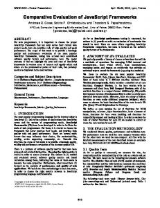
The size of the training set constitutes a significant factor in the overall performance of the trained classifier. In general, the quality of the computed model improves as the size of the training set increases. At the same time, however, the size of the training set is limited by main memory constraints and the time complexity of the learning algorithm. To determine a good data partitioning scheme for the credit card data sets we applied the five learning algorithms over training sets of varying size. The objective was to compute base classifiers with good performance in a “reasonable” amount of time. Specifically, we constructed training sets of varying size, starting from 100 examples to 200,000 examples for both credit card data sets. The accuracy, the TP-FP spread and the savings reported in Figure 1, are the averages of each base classifier after a 10-fold cross-validation experiment. The top row corresponds to classifiers trained over the Chase data set and the bottom row to the First Union data set. Training sets larger than 250,000 examples were too large to fit in the main memory of a 300 MHz PC with 128MB capacity running Solaris 2.6. Moreover, the training of base classifiers from 200,000 examples
7
Average accuracy of Chase classifiers
Average TP-FP spread of Chase classifiers
0.89
Average savings of Chase classifiers
0.55
0.88
900000 800000
0.5
0.87
700000 0.45 600000
0.84
0.4
Sabings
0.85
TP-FP
Accuracy
0.86
0.35
0.83
400000 300000
0.3 0.82
Bayes C4.5 CART ID3 Ripper
0.81
Bayes C4.5 CART ID3 Ripper
0.25
0.8 50000
100000 150000 Size of training file Average accuracy of First Union classifiers
200000
100000 0
0
50000
100000 150000 Size of training file Average TP-FP spread of First Union classifiers
200000
0
0.96
0.8
850000
0.95
0.75
800000
0.7
Bayes C4.5 CART ID3 Ripper
0.93
0.6 TP-FP
0.92 0.91
100000 150000 Size of training file Average savings of First Union classifiers
650000
0.55 0.5
200000
Bayes C4.5 CART ID3 Ripper
700000
600000 550000
0.45
500000
0.4
450000
0.35
400000
0.88
0.3
350000
0.87
0.25
0.9
50000
750000
Bayes C4.5 CART ID3 Ripper
0.65
Savings
0.94
Bayes C4.5 CART ID3 Ripper
200000
0.2 0
Accuracy
500000
0.89
0
50000
100000 Size of training file
150000
200000
300000 0
50000
100000 Size of training file
150000
200000
0
50000
100000 Size of training file
150000
Figure 1: Accuracy (left), TP-FP (center) and savings (right) of the Chase (top row) and the First Union (bottom row) classifiers as a function of the size of the training set.
required several CPU hours anyway, which prevented us from experimenting with larger sets. According to these figures, different learning algorithm perform best for different evaluation metrics and for different training set sizes. Some notable examples include the ID3 algorithm that computes good decision trees over the First Union data and bad decision trees over the Chase data, and Naive Bayes that generates classifiers that are very effective according to the TP-FP spread and the cost model over the Chase data, but does not perform as well with respect to overall accuracy. The Ripper algorithm ranks among the best performers. The graphs show that larger training sets result in better classification models, thus verifying Catlett’s results [3, 4] pertaining to the negative impact of sampling on the accuracy of learning algorithms. On the other hand, 8
200000
they also show that performance curves converge, thus indicating reduced benefits as more data are used for learning. Increasing the amount of training data beyond a certain point may not necessarily provide performance improvements that are significant enough to justify the use of additional system resources to learn over larger data sets. In a related study, Oates and Jensen [24] find that increasing the amount of training data to build classification models often results in a linear increase in the size of the model with no significant improvement in their accuracy. The empirical evidence suggests that there is a tradeoff between the efficient training and the effective training of classifiers. Based on these curves for this data and learning task, the turning point lies between 40,000 and 50,000 examples (i.e. above this point, predictive performance improves very slowly). We decided to partition the credit card data in 12 sets of 42,000 records each, a scheme which (roughly) corresponds to partitioning transaction data by month.
5
Evaluation of Meta-Learning Strategies
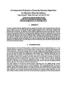
Computing Base Classifiers The first step involves the training of the base classifiers. We distribute each data set across six different data sites (each site storing two subsets) and apply the 5 learning algorithms on each subset of data, therefore creating 60 classifiers (10 classifiers per data site). Next, each data site imports all “remote” base classifiers (50 in total) to test them against its “local” data. In essence, each classifier is evaluated on 5 different (and unseen) subsets. Figure 2 presents the averaged results for the Chase (top row) and First Union (bottom row) credit card data, respectively. The left plots show the accuracy, the center plots depict the TP-FP spread and the right plots display the savings of each base classifier according to the cost model. The x-axis represents the base classifiers, and each vertical bar corresponds to a single model (60 in total). The first set of 12 bars denotes Bayesian classifiers, the second set of 12 bars denotes C4.5 classifiers etc. Each bar in an adjacent group of 12 bars corresponds to a specific subset used to train the classifiers. For example, the first bar of the left plot of the top row of Figure 2 represents the accuracy (83.5%) of the Bayesian classifier that was trained on the first data subset, the second bar represents the accuracy (82.7%) of the Bayesian classifier that was trained on the second data subset and the 13th bar of the 9
Average accuracy of Chase base classifiers
Average TP - FP spread of Chase base classifiers
0.89
Average savings of Chase base classifiers
0.6
Bayes C45 0.88 CART ID3 0.87 Ripper
900000 Bayes C45 CART ID3 Ripper
0.55 0.5
700000 600000
0.84 0.83
Savings
0.45
0.85 TP-FP
Accuracy
0.86
0.4
500000 400000
0.35 300000
0.82 0.3
200000
0.81 0.25
0.8 0.79
100000
0.2 0
10
20
30 40 50 Base Classifiers Average accuracy of First Union base classifiers
60
0 0
0.955
10
20
30 40 50 Base Classifiers Average TP - FP spread of First Union base classifiers
60
0
0.8
Bayes C45 0.945 CART ID3 0.94 Ripper
0.925 0.92
60
Bayes C45 CART ID3 750000 Ripper 700000 Savings
TP-FP
0.93
20 30 40 50 Base Classifiers Average savings of First Union base classifiers
800000
0.65
0.935
10
850000
Bayes 0.75 C45 CART ID3 0.7 Ripper
0.95
Accuracy
Bayes C45 CART ID3 Ripper
800000
0.6 0.55
650000 600000
0.5
550000
0.45
500000
0.4
450000
0.915 0.91 0.905 0.9 0
10
20
30 40 Base Classifiers
50
60
0.35 Dec May Oct Mar Aug Jan Jun Nov Apr Sep Feb Jul Dec Base Classifiers
400000 Dec May Oct Mar Aug Jan Jun Nov Apr Sep Feb Jul Dec Base Classifiers
Figure 2: Fraud Predictors: Accuracy (left), TP-FP spread (middle) and Savings (right) on Chase (top row) and First Union data (bottom row).
same plot (the first of the second group of 12 adjacent bars) represents the accuracy 86.8% of the C4.5 classifier that was trained on the first subset. The maximum achievable savings for the perfect classifier, with respect to our cost model, is $1,470K for the Chase and $1,085K for the First Union data sets. According to the figures, some learning algorithms are more suitable under one problem for one evaluation metric (e.g naive Bayes on Chase data is more effective in savings) than for another metric (e.g. accuracy of naive Bayes classifier on Chase data) or another problem (e.g. naive Bayes on First Union data), even though the two training sets are similar in nature. Overall, it appears that all learning algorithms performed better on the First Union data set than on the Chase data set. On the other hand, note that there are fewer fraudulent transactions in the First Union data and this causes a higher baseline accuracy. In all cases, classifiers are successful in 10
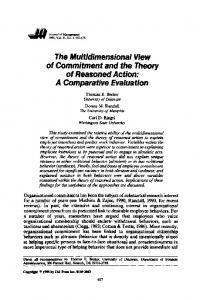
Table 1: Performance of the meta-classifiers Algorithm Majority Weighted Bayes C4.5 CART ID3 Ripper SCANN
Accuracy 89.58% 89.59% 88.65% 89.30% 88.67% 87.19% 89.66% 89.75%
Chase TP-FP 0.556 0.560 0.621 0.567 0.552 0.532 0.585 0.581
Savings $ 596K $ 664K $ 818K $ 588K $ 594K $ 561K $ 640K $ 632K
First Union Accuracy TP-FP 96.16% 0.753 96.19% 0.737 96.21% 0.831 96.25% 0.791 96.24% 0.798 95.72% 0.790 96.53% 0.817 96.53% 0.817
Savings $ 798K $ 823K $ 944K $ 878K $ 871K $ 858K $ 899K $ 899K
detecting fraudulent transactions. Next, we combine these separately learned classifiers under the three different strategies hoping to generate meta-classifiers with improved fraud detection capabilities. Combining Base Classifiers Although the sites are populated with 60 classification models, in meta-learning they combine only the 50 “imported” base classifiers. Since each site uses its local data to meta-learn (the first subset as the validation set and the second subset as the test set) it avoids using the 10 “local” base classifiers to ensure that no classifiers predict on their own training data. We applied 8 different meta-learning methods at each site: the 2 voting strategies (majority and weighted), 5 stacking strategies corresponding to the 5 learning algorithms each used as a meta-learner, and SCANN. Since all sites meta-learn the base classifiers independently, the setting of this experiment corresponds to a 6-fold cross validation with each fold executed in parallel. The performance results of these meta-classifiers averaged over the 6 sites are reported in Table 1. As with the base classifiers, none of the meta-learning strategies outperform the rest in all cases. It is possible, however, to identify SCANN and Ripper as the most accurate meta-classifiers and Bayes as the best performer according to the TP-FP spread and the cost model. (The best result in every category is depicted in bold.) An unexpected outcome of these experiments is the inferior performance of the weighted voting strategy with respect to the TP-FP spread and the cost model. Stacking and SCANN are at a disadvantage since their combining method is ill-defined. Training classifiers to distinguish fraudulent transactions is not a direct approach to maximizing savings (or the TP-FP spread). 11
Traditional learning algorithms are unaware of the adopted cost model and the actual value (in dollars) of the fraud/legitimate label; instead they are designed to reduce misclassification error. Hence, the most accurate classifiers are not necessarily the most cost effective. This can be demonstrated in Figure 2 (top row). Although the Bayesian base classifiers are less accurate than the Ripper and C4.5 base classifiers, they are by far the best under the cost model. Similarly, the meta-classifiers in stacking and SCANN are trained to maximize the overall accuracy not by examining the savings in dollars but by relying on the predictions of the base-classifiers. In fact, the right plot of the top row of Figure 2 reveals that with only a few exceptions, Chase base classifiers are inclined towards catching “cheap” fraudulent transactions and for this they exhibit low savings scores. Naturally, the meta-classifiers are trained to trust the wrong base-classifiers for the wrong reasons, i.e. they trust the base classifiers that are most accurate instead of the classifiers that accrue highest savings. Although weighted voting combines classifiers that too are unaware of the cost model, its meta-learning stage is independent of learning algorithms and hence it is not ill-defined. Instead, it assigns a different degree of influence to each base classifier according to its performance (accuracy, TP-FP spread, savings). Hence, the collective prediction is generated by trusting the best classifiers as determined by the chosen evaluation metric over the validation set. One way to deal with such ill-defined problems is to use cost-sensitive algorithms, i.e. algorithms that employ cost models to guide the learning strategy [25]. On the other hand, this approach has the disadvantage of requiring significant change to generic algorithms. An alternative, but (probably) less effective technique is to alter the class distribution in the training set [2, 7] or to tune the learning problem according to the adopted cost model. In the credit card fraud domain, for example, we can transform the binary classification problem into a multi-class problem by multiplexing the binary class with the continuous amt attribute (properly quantized into several “bins”). A third option, complementary to the other two, is to have the meta-classifier pruned [17], i.e. discard the base classifiers that do not exhibit the desired property. To improve the performance of our meta-classifiers, we followed the latter approach. Although it addresses the cost-model problem at a late stage, after base classifiers are generated, is has the advantage of treating classifiers 12
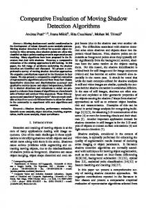
Table 2: Performance of the best pruned meta-classifiers Algorithm Bayes C4.5 CART ID3 Ripper SCANN Majority Weighted
Accur. 89.33% 89.58% 89.49% 89.40% 89.70% 89.76% 89.60% 89.60%
K 16 14 9 8 46 46 47 48
Chase TP-FP 0.632 0.572 0.571 0.568 0.595 0.574 0.577 0.577
K 32 27 18 1 47 32 11 11
Savings $ 903K $ 793K $ 798K $ 792K $ 858K $ 880K $ 902K $ 905K
K 5 5 5 5 3 5 3 4
Accur. 96.57% 96.51% 96.48% 96.45% 96.59% 96.45% 96.55% 96.59%
K 13 16 12 8 30 49 15 12
First Union TP-FP K 0.848 12 0.799 25 0.801 29 0.795 30 0.821 36 0.794 12 0.780 15 0.789 12
Savings $ 950K $ 880K $ 884K $ 872K $ 902K $ 902K $ 854K $ 862K
as black boxes. Furthermore, it can prove invaluable to the computationally and memory expensive SCANN algorithm. To meta-learn 50 classifiers over a 42,000 large validation set, for example, SCANN exhausted the available resources of the 300MHz PC with 128MB main memory and 465MB swap space. By discarding classifiers prior to meta-learning, pruning helps reduce the size of the SCANN meta-learning matrix and naturally simplifies the problem. Pruning Meta-Classifiers Determining the optimal set of classifiers for meta-learning is a combinatorial problem. With 50 base classifiers per data site, there are 250 combinations of base classifiers that can be selected. To search the space of the potentially most promising meta-classifiers, the pruning algorithms [17] employ evaluation functions that are based on the evaluation metric adopted (e.g. accuracy, cost model) and heuristic methods that are based on the performance and properties of the available set of base classifiers (e.g. diversity or high accuracy for a specific class). Table 2 displays the performance results of the best pruned meta-classifiers and their size K (number of constituent base classifiers). Again, there is no single best meta-classifier (best results depicted in bold); depending on the evaluation criteria and the learning task, different meta-classifiers of different sizes perform better. By selecting the base classifiers, pruning helps address the cost-model problem as well as the TP-FP spread problem. The performance of a meta-classifier is directly related to the properties and characteristics of its constituent base classifiers. Recall (from the right plot of the top row of Figure 2) that very few base classifiers from Chase have the ability to catch “expensive” fraudulent transactions. By combining all these classifiers, the meta-classifiers exhibit substantially improved performance (see the savings column of the Chase data in Table 2). This characteristic is not as apparent for the First Union data set since the majority of the First Union base classifiers 13
K 29 42 37 40 44 12 13 10
happened to catch the “expensive” fraudulent transactions anyway (right plot of the bottom row of Figure 2). The same, but to a lesser degree, holds for the TP-FP spread.
6
Concluding Remarks
Integrating multiple learned classification models (classifiers) computed over large and (physically) distributed data sets has been proposed as an effective approach to scaling inductive learning techniques. In this paper we compared the predictive performance and scalability of three commonly-used modelcombining strategies, Voting, Stacking and SCANN (Stacking with Correspondence Analysis) through experiments performed on two databases of actual credit card data, where the learning task is fraud detection. We evaluated the meta-learning methods from two perspectives, their predictive performance (i.e. accuracy, TP-FP spread, savings) and their scalability. For the former, the experiments on the credit card transaction data revealed that there in no single meta-learning algorithm that is best over all cases, although SCANN, stacking with Naive Bayes and stacking with Ripper had an edge. For the latter, the voting methods scale better, while stacking methods depend on the scalability of the meta-learning algorithms (the particular algorithm used for combining models). At the opposite end, SCANN is main memory expensive and has a time complexity of O(M · K)3 (M: number of classes, K: number of base classifiers), making it much less scalable. However, in all cases, the combined meta-classifiers outperformed the base classifiers trained on the largest possible sample of the data. The manner in which the original data set is partitioned into subsets, constitutes a significant parameter to the success of the model-combining (or meta-learning) method. To acquire effective base classifiers efficiently, the size of each subset has to be large enough for the learner to converge to a good model and small enough to allow training under reasonable time and space constraints. There has been extensive analytical research within the Computational Learning Theory(COLT) [1, 12] on bounding the sample complexity using the PAC model [26], the VC dimension [27], Information theory [10] and statistical physics [23]. In this paper, we studied the problem from an experimental perspective in order to determine whether any consistent pattern is discernable, that then may be compared to possible theoretical predictions. Unfortunately, the reported compendium of results demonstrates that there 14
are no specific guideposts indicating the best partitioning strategy and significant experimentation is required to find the best partitioning scheme and meta-learning strategy, under different performance metrics, that scales well. This experiment highlights the need for new research into this important practical issue.
7
Acknowledgments
We are in debt to Chris Merz for providing us with his implementation of the SCANN algorithm.
References [1] M. Anthony and N. Biggs. Computational learning theory: An Introduction. Cambridge University Press, Cambridge, England, 1992. [2] L. Breiman, J. H. Friedman, R. A. Olshen, and C. J. Stone. Classification and Regression Trees. Wadsworth, Belmont, CA, 1984. [3] J. Catlett. Megainduction: A test flight. In Proc. Eighth Intl. Work. Machine Learning, pages 596–599, 1991. [4] J. Catlett. Megainduction: machine learning on very large databases. PhD thesis, Dept. of Computer Sci., Univ. of Sydney, Sydney, Australia, 1992. [5] P. Chan and S. Stolfo. Meta-learning for multistrategy and parallel learning. In Proc. Second Intl. Work. Multistrategy Learning, pages 150–165, 1993. [6] P. Chan and S. Stolfo. A comparative evaluation of voting and meta-learning on partitioned data. In Proc. Twelfth Intl. Conf. Machine Learning, pages 90–98, 1995. [7] P. Chan and S. Stolfo. Toward scalable learning with non-uniform class and cost distributions: A case study in credit card fraud detection. In Proc. Fourth Intl. Conf. Knowledge Discovery and Data Mining, pages 164–168, 1998. [8] P. Chan, S. Stolfo, and D. Wolpert, editors. Working Notes for the AAAI-96 Workshop on Integrating Multiple Learned Models for Improving and Scaling Machine Learning Algorithms, Portland, OR, 1996. AAAI. [9] W. Cohen. Fast effective rule induction. In Proc. 12th Intl. Conf. Machine Learning, pages 115–123, 1995. [10] M. Kearns D. Haussler and R. E. Shapire. Bounds on the sample complexity of bayesian learning using information theory and the vc dimension. Machine Learning, 14:83–113, 1994. [11] Michael J. Greenacre. Theory and Application of Correspondence Analysis. Academic Press, London, 1984.
15
[12] M. J. Kearns and U.V. Vazirani. An Introduction to computational learning theory. MIT Press, Cambridge, MA, 1994. [13] N. Littlestone and M. Warmuth. The weighted majority algorithm. Technical Report UCSC-CRL-89-16, Computer Research Lab., Univ. of California, Santa Cruz, CA, 1989. [14] C. Merz. Using correspondence analysis to combine classifiers. Machine Learning, 1998. to appear. [15] M. Minksy and S. Papert. Perceptrons: An Introduction to Computation Geometry. MIT Press, Cambridge, MA, 1969. (Expanded edition, 1988). [16] A. L. Prodromidis and S. J. Stolfo. Agent-based distributed learning applied to fraud detection. In Sixteenth National Conference on Artificial Intelligence. Submitted for publication. [17] A. L. Prodromidis and S. J. Stolfo. Pruning meta-classifiers in a distributed data mining system. In In Proc of the First National Conference on New Information Technologies, pages 151–160, Athens, Greece, October 1998. [18] F. Provost and T. Fawcett. Analysis and visualization of classifier performance: Comparison under imprecise class and cost distributions. In Proc. Third Intl. Conf. Knowledge Discovery and Data Mining, pages 43–48, 1997. [19] F. Provost and T. Fawcett. Robust classification systems for imprecise environments. In Proc. AAAI-98. AAAI Press, 1998. [20] F. Provost and V. Kolluri. Scaling up inductive algorithms: An overview. In Proc. Third Intl. Conf. Knowledge Discovery and Data Mining, pages 239–242, 1997. [21] J. R. Quinlan. Induction of decision trees. Machine Learning, 1:81–106, 1986. [22] J. R. Quinlan. C4.5: programs for machine learning. Morgan Kaufmann, San Mateo, CA, 1993. [23] H. S. Seung, H. Sompolinsky, and N. Tishby. Statistical mechanics of learning from examples. Physical Review, A45:6056–6091, 1992. [24] D. Jensen T. Oates. Large datasets lead to overly complex models: As explanation and a solution. In G. Piatetsky-Shapiro R. Agrawal, P. Stolorz, editor, Proc. Fourth Intl. Conf. Knowledge Discovery and Data Mining, pages 294–298. AAAI Press, 1998. [25] P. D. Turney. Cost-sensitive classification: Empirical evaluation of a hydrid genetic decision tree induction algorithm. Journal of AI Research, 2:369–409, 1995. [26] L. Valiant. A theory of the learnable. Comm. ACM, 27:1134–1142, 1984. [27] V. N. Vapnik and A. Chervonenkis. On the uniform convergence of relative frequencies of events to their posibilities. Theory of Probability and Its Applications, 16:264–280, 1971. [28] D. Wolpert. Stacked generalization. Neural Networks, 5:241–259, 1992.
16