A comparative study of local descriptors for object category - VisLab

3rd Iberian Conference on Pattern Recognition and Image Analysis, Girona, Spain, June 2007

A comparative study of local descriptors for object category recognition: SIFT vs HMAX Plinio Moreno1 , Manuel J. Mar´ın-Jim´enez2 , Alexandre Bernardino1 , Jos´e Santos-Victor1 , and Nicol´as P´erez de la Blanca2 1

2

Instituto Superior T´ecnico & Instituto de Sistemas e Rob´ otica 1049-001 Lisboa - Portugal Dpt. Computer Science and Artificial Intelligence, University of Granada, ETSI Inform´ atica y Telecomunicaci´ on, Granada, 18071, Spain [email protected], [email protected], [email protected], [email protected], [email protected]

Abstract. In this paper we evaluate the performance of the two most successful state-of-the-art descriptors, applied to the task of visual object detection and localization in images. In the first experiment we use these descriptors, combined with binary classifiers, to test the presence/absence of object in a target image. In the second experiment, we try to locate faces in images, by using a structural model. The results show that HMAX performs slightly better than SIFT in these tasks.

1

Introduction

A key issue in visual object recognition is the choice of an adequate local descriptor. Recently Mikolajczyk et al. [1] presented a framework to compare local descriptor performance in image region matching. However, their conclusions are not guaranteed to be valid in object category recognition. Thus, in this work we perform a comparative study of two of the most successful state-of-the-art local descriptors (SIFT and HMAX), applied to object category detection and localization in images. We aim to use the same experimental set-up, to evaluate the actual impact of local descriptor choice. Scale Invariant Feature Transform (SIFT) [2] is a location-histogram-based descriptor, very successful in single object recognition. Among the several extensions to SIFT descriptor, SIFT-Gabor [3] improves SIFT matching properties, and is also used in this work. On the other side, the biologically inspired descriptor HMAX [4] which combines the information of several filters and max operators, has shown excellent performance in object category recognition. We perform experiments with two kinds of object models: (i) appearance only, and (ii) shape and appearance. In the first group of experiments we model objects by a bunch of local descriptors. In this model we disregard descriptor’s location information, so we are able to decide object presence/absence in new images, but is not possible to estimate object position in the image. We detect 1

nine different object categories, considering each category recognition as a twoclass problem (object samples and background samples). In order to estimate class models, we use AdaBoost and SVM learning algorithms. In the second group of experiments, we model objects using local descriptors as appearance and pictorial structure as shape model. This shape model represents an object as a star-like graph. The graph nodes correspond to image region local descriptors (appearances), and edges connect pairs of nodes whose relative location can be modelled by a two dimensional Gaussian (object shape). With this model we are able to decide object presence/absence and location in new images. This model allows object translations, and is robust to small scalings, but it is not fully invariant to object rotations and scalings. This paper is organized as follows: in Section 2, SIFT and HMAX descriptors are briefly introduced. Then, in Section 3, we describe the object shape model. Afterwards, the experiments and results are presented in Sections 4 and 5. And, finally, we conclude the paper with the summary and conclusions.

2

Appearance models

In order to compute region appearance models, we compute three descriptors: SIFT, SIFT-Gabor modification and HMAX. 2.1

SIFT descriptor

In the original formulation of the SIFT descriptor [2], a scale-normalized image region is represented with the concatenation of gradient orientation histograms relative to several rectangular subregions. Firstly, the derivatives Ix and Iy of the image I are computed with pixel differences. Then the image gradient magnitude and orientation is computed for every pixel in the scale-normalized image region: q M (x, y) = Ix (x, y)2 + Iy (x, y)2 ; Θ(x, y) = tan−1 (Iy (x, y)/Ix (x, y)). (1) The interest region is then subdivided in subregions in a rectangular grid. The next step is to compute the histogram of gradient orientation, weighted by gradient magnitude, for each subregion. Orientation is divided into B bins and each bin is set with the sum of the windowed orientation difference to the bin center, weighted by the gradient magnitude: X M (x, y)(1 − |Θ(x, y) − ck |/∆k ), (2) hr(l,m) (k) = x,y∈r(l,m)

where ck is the orientation bin center, ∆k is the orientation bin width, and (x, y) are pixel coordinates in subregion r(l,m) . The SIFT local descriptor is the concatenation of the several gradient orientation histograms for all subregions: u = (hr(1,1) , . . . , hr(l,m) , . . . , hr(4,4) )

(3)

With 16 subregions and B = 8 orientations bins, u size is 128. The final step is to normalize the descriptor in Eq.(3) to unit norm, in order to reduce the effects of uniform illumination changes. 2

SIFT-Gabor descriptor Using the framework provided by Mikolajcyzik et al. [1], we improve SIFT distinctiveness for image region matching. We propose an alternative way to compute first order image derivatives using odd Gabor filters, instead of pixel differences [3]. We rely on filter energy, to select the most appropriate Gabor filter width especially suited to represent scale-normalized image regions. Image derivatives are computed as odd √ )(x, y); Ix (x, y) = (I ∗ g0,6,4 2/3

odd √ Iy (x, y) = (I ∗ gπ/2,6,4 )(x, y). 2/3

(4)

odd where gθ,γ,σ (x, y) is the 2D odd Gabor function with orientation θ, scale invariant wave number γ, and width σ. Once the image derivatives are computed, we do as original SIFT histogram computation.

2.2

HMAX model

The biologically inspired HMAX model was firstly proposed by Riesenhuber and Poggio [4], and lately revised by Serre et al. [5], who introduced a learning step based on the extraction of lots of random patches. On the latter version, Mar´ınJim´enez and P´erez de la Blanca [6] have proposed some changes that we have adopted for this work, in particular, the use of Gaussian derivatives functions (i.e. second order) instead of Gabor functions. We include a brief description of the steps of the HMAX model to generate C2 features (see [5] for details): 1. Compute S1 maps: the target image is convolved with a bank of oriented filters with various scales. 2. Compute C1 maps: pairs of S1 maps (of different scales) are subsampled and combined, by using the max operator, to generate bands. 3. Only during training: extract patches Pi of various sizes ni × ni and all orientations from C1 maps, at random positions. 4. Compute S2 maps: for each C1 map, compute the correlation Y with the patches Pi : Y = exp(−γkX − Pi k2 ), where X are all the possible windows in C1 with the same size as Pi , γ is a tunable parameter. 5. Compute C2 features: compute the max over all positions and bands for each S2i map, obtaining a single value C2i for each patch Pi .

3

Object Shape model

The objects are composed by a set of P parts, and modelled by the relative locations between parts and appearance of every part. The locations between parts is a star-like graph, where the star’s reference point (landmark) must be present in the image in order to detect an object. The pictorial model is parametrized by the graph G = (V, E). V = {v1 , . . . , vp , . . . , vP } is the set of vertices and v1 is the landmark point. E = {e12 , . . . , e1p , . . . , e1P } is the set of edges between connected parts, where e1p denotes the edge connecting part 1 and part p. We model the edge parameters as Gaussian distributions of the 3

x and y coordinates referenced to the landmark location. The edge model is e1p = (µxp −x1 , σx2p −x1 , µyp −y1 , σy2p −y1 ), p = 2, . . . , P ; e1p ∈ E, where the mean(µ) and variance(σ 2 ) are estimated in the training set. Additionally to edge parameters, the set of appearance models related to vertices is u = {u1 , . . . , up , . . . , uP }. The statistical framework proposed in [7], computes the probability of an object configuration L = {l1 , . . . , lp , . . . , lP }, li = (xp , yp ), given an image3 I and a model θ = (u, E) as p(L|I, θ) ∝ p(I|L, θ)p(L|θ). (5) Assuming non-overlapping parts in the object, the likelihood of I given the configuration L and model θ can be approximated by the product of probabilities QP of each part, so p(I|L, θ) = p(I|L, u) ∝ p=1 p(I|lp , up ). The prior p(L|θ) is captured by the Markov random field with edge set E.Q Following the reasoning proposed in [7], the prior is approximated by p(L|θ) = e1p ∈E p(x1 , xp |θ)p(y1 , yp |θ). Thus replacing the likelihood and prior in Eq. (5), and computing the negative logarithm, the best object configuration is

L∗ = arg min − L

P X p=1

log p(I|lp , up )−

X

log p(x1 , xp |cp )−

(e1p ∈E)

X

log p(y1 , yp |cp ).

(e1p ∈E)

(6) The Eq.(6) computes in a new image I the most probable configuration L∗ , after learning the model θ = (u, E).

4

Object Detection Experiment

In this group of experiments we model an object category by a set of local descriptors (SIFT/HMAX). We select N points from training set images of object class c, and compute local descriptor uci at selected point i. With SIFT descriptors, u is the gradient histogram vector in Eq. (3) and, with HMAX descriptor u is the patch Pi described in Section 2.2. During training, for all cases, we select points searching for local maxima of Difference of Gaussians (DoG), but in original HMAX points are selected at random. In order to detect an instance of the category modelled in a new image we: 1. Select J interest point locations by applying DoG operator. But in original HMAX, all the image points are candidates (see section 2.2 ). 2. Compute local descriptors in the new image uj , j = 1, . . . , J at interest point locations. 3. Create class-similarity feature vector v = [v1 , . . . , vi , . . . , vN ] by matching each class model point descriptor uci against all image descriptors uj . In the 2 case of SIFT descriptor vi = minj kuci − uj k , and in the case of HMAX descriptor vi = maxj exp(−γkPi − uj k2 ). 4. Classify v as object or background image, with a binary classifier. 4

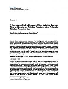
Fig. 1. Typical images from selected databases.

The experiments are performed over a set of classes provided by Caltech 4 : airplanes side, cars side, cars rear, camels, faces, guitars, leaves, leopards and motorbikes side, plus Google things dataset [8]. We use category Google things as negative samples. Each positive training set is comprised of 100 images drawn at random, and 100 images drawn at random from the unseen samples for testing. Figure 1 shows some sample images from each category. For all experiments, images have a fixed size (height 140 pixels), keeping the original image aspect ratio and converted to gray-scale format. We vary the number of local descriptors that represent an object category, N = {5, 10, 25, 50, 100, 250, 500}. In order to evaluate the influence of the learning algorithm, we utilize two classifiers: SVM [9] with linear kernel5 , and AdaBoost [11] with decision stumps. The experimental set-up for each kind of local descriptor is: (i) original HMAX, (ii) HMAX computed at DoG, (iii) SIFT non-rotation-invariant (NRI), (iv) original SIFT, (v) SIFT-Gabor, and (vi) SIFT-Gabor NRI. Results and discussion In Table 1, we show the mean results of detection for 10 repetitions at equilibrium point (i.e. when the false positive rate = miss rate), along with confidence interval (at 95%). We only show results for 10 and 500 features. In Fig. 2 we see performance evolution as a function of the number of features, in the case of rigid (airplanes) and articulated (leopards) objects. Local descriptors can be clustered in three groups using the average performance: HMAX-based descriptors, SIFT-NRI descriptors, and SIFT descriptors. HMAX-based descriptors have the best performance, followed by SIFT-NRI descriptors and SIFT descriptors. The separation between the groups depends on the learning algorithm, in the case of SVM the distance between groups is large. In the case of AdaBoost groups are closer to each other, and for some categories (motorbikes, airplanes and leopards) all descriptors have practically the same performance. We see that in average, results provided by SVM are better than the AdaBoost ones. Although in [3] is concluded that SIFT-Gabor descriptor improves SIFT distinctiveness on average for image region matching, we cannot apply this conclusion to object category recognition. In the case of AdaBoost algorithm SIFT and SIFT-Gabor have practically the same performance, while in the case of SVM SIFT performs slightly better than SIFT-Gabor. 3 4 5

set of intensity values that represents visually the object Datasets are available at: http://www.robots.ox.ac.uk/˜vgg/data3.html Implementation provided by libsvm[10]

5

Table 1. Results for all the categories. (TF: type of feature. NF: number of features). On average over all the categories and using SVM, HMAX-Rand gets 84.2%, versus the 73.9% of regular SIFT. For each experiment, the best result is in bold face.

Support Vector Machines Airplane Camel Car-side Car-rear TF/NF 10 500 10 500 10 500 10 500 H-Rand 87.3, 2.2 95.9, 1.0 70.4, 3.1 84.3, 2.2 87.9, 4.0 98.1, 1.5 93.0, 1.1 97.7, 0.8 H-DoG 80.3, 2.6 94.9, 0.8 70.2, 3.9 83.9, 1.4 88.9, 3.8 99.5, 0.9 86.6, 1.8 97.0, 0.7 Sift 74.6, 1.8 89.1, 1.0 63.9, 2.4 76.1, 1.7 72.9, 3.4 87.9, 3.7 73.7, 2.7 88.4, 2.1 G-Sift 69.7, 2.9 88.6, 1.5 57.3, 1.8 77.2, 2.2 69.1, 5.6 87.0, 2.0 67.2, 2.1 85.8, 1.7 SiftNRI 78.0, 3.2 92.4, 1.3 63.1, 3.8 77.8, 1.9 79.2, 3.4 90.8, 2.2 86.9, 1.8 93.1, 1.2 G-SiftNRI 74.8, 2.6 92.8, 1.5 62.1, 3.4 75.9, 1.9 72.5, 4.9 87.4, 2.2 80.2, 1.9 90.7, 1.2 Faces Guitar Leaves Leopard Motorbike 10 500 10 500 10 500 10 500 10 500 79.8, 3.4 96.6, 0.7 87.1, 4.0 96.7, 1.1 88.6, 3.1 98.3, 0.6 81.4, 3.4 95.7, 0.9 81.9, 3.4 93.7, 0.9 82.7, 1.8 96.0, 0.6 82.9, 4.0 95.9, 0.8 84.6, 2.0 98.3, 0.9 70.9, 3.9 94.2, 1.3 81.6, 2.3 94.7, 0.7 74.8, 3.3 88.4, 1.8 66.4, 3.0 81.1, 1.5 81.5, 3.5 92.6, 1.1 81.7, 2.5 87.8, 1.1 75.2, 2.3 87.9, 1.4 73.6, 2.9 85.2, 1.9 70.1, 1.9 82.3, 1.1 81.0, 3.3 92.4, 1.0 78.0, 3.0 89.6, 1.3 69.0, 2.6 86.9, 1.4 84.4, 3.4 92.8, 1.2 65.2, 3.3 85.4, 1.0 79.1, 2.8 92.6, 0.9 81.6, 1.7 92.4, 1.2 75.4, 2.4 90.9, 1.7 84.6, 3.3 91.8, 1.2 69.0, 3.8 86.1, 1.6 79.1, 3.3 91.7, 1.3 76.9, 3.2 91.8, 1.4 72.0, 2.9 89.6, 0.7 AdaBoost Airplane Camel Car-side Car-rear TF/NF 10 500 10 500 10 500 10 500 H-Rand 81.0, 0.7 94.3, 1.1 67.7, 3.3 83.1, 1.0 84.1, 2.8 94.2, 2.0 90.1, 5.1 98.3, 0.7 H-DoG 77.8, 3.6 93.2, 1.3 63.9, 4.5 79.1, 1.8 85.5, 5.5 96.6, 1.3 74.1, 15.7 96.4, 1.3 Sift 75.3, 3.3 90.6, 1.5 65.1, 1.9 73.8, 1.6 74.9, 4.0 88.9, 2.1 76.3, 2.6 89.8, 1.6 G-Sift 73.0, 4.1 90.2, 1.2 60.6, 2.4 77.3, 2.0 70.5, 4.7 87.0, 3.5 69.7, 1.5 87.2, 2.0 SiftNRI 79.8, 3.2 93.1, 1.1 65.0, 3.4 78.1, 1.5 81.6, 4.9 90.8, 2.2 89.6, 0.7 94.9, 1.2 G-SiftNRI 77.9, 2.4 94.2, 1.2 62.2, 2.9 74.8, 2.3 78.3, 3.8 89.9, 2.0 83.8, 1.3 92.3, 0.9 Faces Guitar Leaves Leopard Motorbike 10 500 10 500 10 500 10 500 10 500 77.1, 4.7 94.9, 1.1 83.7, 7.1 96.6, 1.0 83.1, 6.2 97.7, 0.7 76.8, 2.8 85.6, 1.1 74.7, 4.8 92.0, 1.7 74.4, 6.1 95.7, 1.2 78.0, 6.9 92.7, 1.5 76.0, 4.6 97.0, 0.9 70.2, 5.5 83.1, 2.0 75.2, 3.7 93.4, 0.9 78.3, 3.1 90.8, 1.2 66.0, 3.4 79.9, 1.1 84.2, 3.2 92.6, 1.1 83.6, 2.2 87.0, 1.2 77.9, 1.7 90.7, 1.4 75.3, 3.3 87.4, 1.7 71.6, 2.6 83.4, 2.6 81.1, 4.3 92.9, 1.3 81.2, 1.8 89.7, 2.2 70.8, 2.9 88.9, 1.2 87.6, 2.7 94.3, 0.8 67.2, 2.8 86.4, 1.4 81.0, 3.6 92.9, 1.5 84.4, 1.5 92.8, 1.2 80.4, 2.6 93.7, 1.1 86.1, 2.8 92.6, 1.3 69.9, 4.3 87.4, 1.0 81.7, 3.8 92.2, 1.9 78.1, 1.9 91.7, 1.0 75.4, 2.3 92.3, 1.2

HMAX is able to discriminate categories, attaining rates over 80% in most of the cases with a small number of features, e.g. 10. It shows that a discriminative descriptor can detect objects in categories with very high visual difficult images, like leopards and camels, using an appearance model. Other remarkable data is that HMAX-DoG works better with car-side and motorbikes, since DoG operator is able to locate the most representative parts, e.g. the wheels.

5

Face detection and localization experiment

The aim of this experiment is to detect and locate faces in images using appearance models (SIFT and HMAX) and shape model (pictorial structure). We use a subset of the Caltech faces (100 images), background (100 images) database images, and the software provided at the “ICCV’05 Short Course” [12]. Here it is important to remark that background images do not model a negative class, but 6

Performance (SVM): leopards

100

95

95

90

90

85

85 %

%

Performance (SVM): airplanesside

100

80 75

75

70

70 HMAX−RAND HMAX−SIFT SIFT128 SIFT128Gabor SIFT128NRI GaborSIFT128NRI

65 60 0

80

100

200 300 N features

400

HMAX−RAND HMAX−SIFT SIFT128 SIFT128Gabor SIFT128NRI GaborSIFT128NRI

65

500

60 0

100

200 300 N features

400

500

Fig. 2. Comparison of performance depending on the type and number of features representing the images. The used classifier is SVM.

Fig. 3. Face detection samples: 3 hits and 1 miss (right).

they are utilized only to test the object model in images without faces. We select 10% of the face images to learn the local descriptor model (µup , Σup ), and the pictorial structure model (µxp −x1 , σx2p −x1 , µyp −y1 , σy2p −y1 ), with P = 5 parts. We recognize faces in the remaining 90% of face image set and background images. Results and discussion Evaluation criterion comprises object detection and location. In the case of object detection we compute the Receiver Operator Characteristic (ROC) curve, varying the threshold in L∗ from Eq. (6). In the case of object location we compute precision vs. recall curve (RPC), varying the ratio between the intersection and union of ground truth and detected bounding boxes. From ROC we compute area (A-ROC) and equal error rate point (EEP), and, from RPC we compute equal error rate (RPC-eq) presented in Table 2. The results show that HMAX’s C1-level based descriptors are suitable to represent object parts, achieving better results than SIFT descriptors. Figure 3 shows three correct detections and one wrong detection, when using five parts for the model and HMAX as part descriptor.

Feature Nparts A-ROC EEP RPC-eq HMAX 5 94.8 89.0 84.9 SIFT 5 93.4 86.3 80.3 SIFT-Gabor 5 94.9 85.3 81.7

Table 2. Results for face detection and localization using the structural model.

7

6

Summary and conclusions

We carry out a comparative study of SIFT and HMAX (C1 level) as local descriptors for object recognition. We aim to perform a fair comparison, using the same set-up elements: (i) training and test sets, (ii) object models, and (iii) interest point selection. We evaluate performance of both descriptors in two object models: (i) appearance only, and (ii) shape and appearance. After performing the experiments with different datasets, we see that, on average, disregarding interest point detection, learning algorithm, and object model, HMAX performs better than SIFT in all the different experiments. As future work, in order to evaluate the impact of interest point selection in recognition performance, we intend to evaluate other interest point detectors in this framework. Acknowledgments. This work was partially supported by the Spanish Ministry of Education and Science, grant FPU AP2003-2405 and project TIN200501665, by the FCT Programa Operacional Sociedade de Informa¸c˜ao (POSI) in the frame of QCA III, and Portuguese Foundation for Science and Technology PhD Grant FCT SFRH\BD\10573\2002 and partially supported by Funda¸c˜ao para a Ciˆencia e a Tecnologia (ISR/IST plurianual funding) through the POS Conhecimento Program that includes FEDER funds and FCT Project GestInteract.

References 1. K. Mikolajczyk and C. Schmid. A performance evaluation of local descriptors. IEEE PAMI, 27(10):1615–1630, November 2005. 2. David G. Lowe. Distinctive image features from scale-invariant keypoints. International Journal of Computer Vision, 2(60):91–110, 2004. 3. P. Moreno, A. Bernardino, and J. Santos-Victor. Improving the sift descriptor with gabor filters. Submitted to Pattern Recognition Letters, 2006. 4. M. Riesenhuber and T. Poggio. Hierarchical models of object recognition in cortex. Nature Neuroscience, 2(11):1019–1025, 1999. 5. T. Serre, L. Wolf, and T. Poggio. Object recognition with features inspired by visual cortex. In IEEE CSC on CVPR, June 2005. 6. M.J. Mar´ın-Jim´enez and N. P´erez de la Blanca. Empirical study of multi-scale filter banks for object categorization. In Proc ICPR, pages 578–581, Washington, DC, USA, August 2006. IEEE Computer Society. 7. Pedro F. Felzenszwalb and Daniel P. Huttenlocher. Pictorial structures for object recognition. Intl. J. Computer Vision, 1(61):55–79, Jan 2005. 8. R. Fergus, P. Perona, and A. Zisserman. A sparse object category model for efficient learning and exhaustive recognition. In CVPR, pages 380–387, June 2005. 9. E. Osuna, R. Freund, and F. Girosi. Support Vector Machines: training and applications. Technical Report AI-Memo 1602, MIT, March 1997. 10. C. Chang and C. Lin. LIBSVM: a library for support vector machines, April 2005. 11. J. Friedman, T. Hastie, and R. Tibshirani. Additive logistic regression: a statistical view of boosting. Technical report, Dept. of Statistics. Stanford University, 1998. 12. L. Fei-Fei, R. Fergus, and A. Torralba. http://people.csail.mit.edu/torralba/iccv2005/.

8