Fuzzy C-Means. 1. INTRODUCTION. The standard convex geometry model assumes that an input hyperspectral ... values for a data point must sum to one.
Submitted to the Proc. of the WHISPERS 2010, To Appear.
A COMPARISON OF DETERMINISTIC AND PROBABILISTIC APPROACHES TO ENDMEMBER REPRESENTATION Alina Zare† , Ouiem Bchir∗ , Hichem Frigui∗ , and Paul Gader† †
Department of Computer and Information Science and Engineering, University of Florida ∗ Computer Engineering and Computer Science Department, University of Louisville ABSTRACT
The piece-wise convex multiple model endmember detection algorithm (P-COMMEND) and the Piece-wise Convex Endmember detection (PCE) algorithm autonomously estimate many sets of endmembers to represent a hyperspectral image. A piece-wise convex model with several sets of endmembers is more effective for representing non-convex hyperspectral imagery over the standard convex geometry model (or linear mixing model). The terms of the objective function in P-COMMEND are based on geometric properties of the input data and the endmember estimates. In this paper, the PCOMMEND algorithm is extended to autonomously determine the number of sets of endmembers needed. The number of sets of endmembers, or convex regions, is determined by incorporating the competitive agglomeration algorithm into P-COMMEND. Results are shown comparing the Competitive Agglomeration P-COMMEND (CAP) algorithm to results found using the statistical PCE endmember detection method.
(a)
(b)
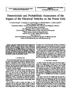
Fig. 1. (a) Band 10 (0.49 µm) of the AVIRIS Indian Pines data set. (b) Scatter plot of the Indian Pines data set after dimensionality reduction to three dimensions using PCA.
Endmember Detection (PCE) algorithm that samples from a Dirichlet process to determine the number of convex regions needed to represent a hyperspectral image.
Index Terms— Hyperspectral, Endmember, Spectral Unmixing, Convex Geometry Model, Linear Mixing Model, Fuzzy C-Means.
In the following, Section 2 outlines the P-COMMEND algorithm, Section 3 introduces the Competitive Agglomeration P-COMMEND (CAP) extension that learns the number of convex regions needed, Section 4 presents experimental results comparing the geometrical CAP method to the statistical PCE method and Section 5 provides a discussion and conclusions.
1. INTRODUCTION The standard convex geometry model assumes that an input hyperspectral image is represented as a single convex region with a single set of endmembers. However, hyperspectral images are often not convex. For example, as shown in Figure 1, the AVIRIS Indian Pines data set is not convex [1]. P-COMMEND [2] represents hyperspectral imagery using several sets of endmembers that allows for a more accurate representation of non-convex hyperspectral images. The piece-wise convex representation for hyperspectral imagery was first developed in [3] and [4] with the Piece-wise Convex
2. P-COMMEND
The P-COMMEND algorithm [2] performs alternating optimization to autonomously estimate the endmembers, E, abundances, P, and membership values, U, for a given hyperspectral image. P-COMMEND iteratively minimizes the objective function in Equation 1 subject to the sum-to-one and non-negativity constraints on the proportions and mem-
Research was supported by NSF program Optimized Multi-algorithm Systems for Detecting Explosive Objects Using Robust Clustering and Choquet Integration (CBET-0730484). The views and conclusions contained in this document are those of the authors and should not be interpreted as representing the official policies, either expressed or implied, of NSF. The U. S. Government is authorized to reproduce and distribute reprints for Government purposes notwithstanding any copyright notation hereon.
1
Submitted to the Proc. of the WHISPERS 2010, To Appear. bership values. J
=
C X N X
and pKKT = max pTij , 0 ij
um ij
T
(xj − pij Ei ) (xj − pij Ei )
where λij = 2
i=1 j=1
+
α
C X
M · trace(Ei ETi ) − 11×M Ei ETi 1M ×1
�
11×M Ei ET i
(
�
(5)
−1
)
Ei xT j −1 −1 1M ×1
11×M (Ei ET i )
.
3. COMPETITIVE AGGLOMERATION P-COMMEND (CAP)
i=1
(1) In order to estimate the number of convex regions needed for an input data set, the Competitive Agglomeration algorithm [9] is integrated into the P-COMMEND algorithm. Competitive Agglomeration uses a term with the sum of the squared membership values. The objective function for CAP is shown in Equation 6.
where xj is a 1×d vector representing the j th pixel of the image, N is the number of pixels in the image, M is the number of endmembers in each convex region, Pi is a N × M matrix such that pij , is the vector of abundances associated with pixel j with respect to model i, and Ei is a M × d matrix such that each row of Ei , eik , is a 1 × d vector representing the k th endmember with respect to model i. The notation 1S×T denotes an S × T matrix with all entries equal to 1. Each set of endmembers compete for data through the uij weights which is the membership xj data in the ith model. The m parameter is the “fuzzifier” controlling the degree to which the data points are shared among the models. The first term of this objective function computes the residual error between the data and their projections into the regions defined by each set of endmembers. The use of the fuzzy membership values is related to the fuzzy c-means algorithm and the Multiple Model General Linear Regression [5, 6]. The second term is sum of squared distances (SSD) between the endmembers and encourages the endmembers to provide a tight fit around the data [7, 8]. For each set of endmembers, both the projection and sum-of-squared distances term is based on the geometry of the data and the estimated endmembers. When updating membership values, the objective function is minimized subject to the constraint that all the membership values for a data point must sum to one. This results in the following update equation given abundances and endmembers, 1
uij = PC
q=1
�
(xj −pij Ei )(xj −pij Ei )T (xj −pqj Eq )(xj −pqj Eq )T
. 1 � m−1
J
T
u2ij (xj − pij Ei ) (xj − pij Ei )
i=1 j=1
+ α
C X
M · trace(Ei ETi ) − 11×M Ei ETi 1M ×1
�
i=1
− β
C X
N X
i=1
2 uij
(6)
j=1
The updates for the endmembers and proportion values remain the same as in P-COMMEND (with a fuzzifier value of 2). The update for the membership values changes as shown in Equation 7. uij = where
βNi + λj
(7)
T
(xj − pij Ei ) (xj − pij Ei )
PC 1 − β k=1 λj = PC
Nk ||xj −pij Ei ||22
(8)
1 k=1 ||xj −pij Ei ||2 2
PN and Nk = j=1 ukj . Competitive agglomeration encourages sparsity in the membership values. When the membership values associated with a single convex region drop below a prescribed threshold, the convex region can be removed. Following the discussion in [9], the β parameter for the competitive agglomeration term is adjusted each iteration using the following schedule.
(2)
The endmembers are updated given the following equation, −1 X X T T (3) Ei = um um ij pij pij + 2αD ij pij xj j
=
C X N X
j
β(t) = β0 e
where D = M IM ×M −1M ×M . Finally, abundance values are updated by minimizing Equation 1 by using a Lagrange multiplier term to enforce the sum-to-one constraints and evaluating and applying the required KKT conditions for the nonnegativity constraints. The resulting update equations are � � �−1 λij pTij = Ei ETi Ei xTj − 1M ×1 (4) 2
−t τ
PC PN i=1
2
u2ij ||xj − pij Ei ||2 � �2 PN PC u i=1 j=1 ij j=1
(9)
where t is the iteration number. This schedule for the β parameter tries to balance the residual error term and the competitive agglomeration term while giving a larger weight the the error term as the number of iterations increase. Future work on CAP will include adjusting the β parameter to take 2
Submitted to the Proc. of the WHISPERS 2010, To Appear. Table 1. Number of Convex Regions estimated using CAP over 1000 runs of the algorithm on the Cuprite data set. Parameter values were held constant. Random initialization was used for each run. Estimated Number of Convex Regions 4 5 6
Fig. 2. Results of CAP on simulated Piece-Wise Convex twodimensional data. into account the sum-squared-distances term on the endmembers as well as the α parameter. A similar schedule for the α parameter will also be developed. In the current implementation of this algorithm, the E, P and U values are randomly initialized and then refined using the fuzzy c-means algorithm.
timated endmembers. As described fully in [4], the statistical properties of PCE that provide this improvement over CAP include a sparsity promoting prior on the abundance values that drive the proportions for un-needed endmembers in convex region to zero and the property that PCE uses a full endmember distribution to represent each endmember rather than a single spectrum. The use of the endmember distributions allow for several unique data points to have a proportion value of 1 associated with the same endmember while controlling the residual error term. However, in comparison to the time needed to run the Gibbs sampling used in PCE, CAP is faster and can easily be applied to large hyperspectral data sets. The difference in running time causes difficulty in comparing the two methods. CAP was easily run on the data 50 times and, due to the slow running time, only a single PCE result was available for comparison. CAP was also applied to the AVIRIS Cuprite “Scene 4” data set. This data contains 51 spectral bands ranging from 1978 to 2477 nm. The quality of the endmembers found can be examined by comparing results to spectra from the USGS spectral library. For direct comparison with the results using PCE in [4], the same data set was used. This data set was generated by selecting candidate points using the pixel purity index (PPI) [10]. From 10,000 random projections in PPI, 1011 pixels were selected as the candidate points. The threshold was set to allow as close to 1000 pixels as possible (several points had the same PPI value). The parameter set used for these experiments were α = 0.1, β0 = 3, τ = 5, and M = 3. In order to determine the quality of the endmembers, they were compared to 100 USGS spectra materials known to be found in the scene: Alunite, Buddingtonite, Calcite, Chalcedony, Desert Varnish, Kaolinite, Montmorillonite, Muscovite, Nontrite and Sphene. The Euclidean distance between the normalized truth and estimated endmembers were computed for one random initialization of this algorithm. Table 2 shows these Euclidean distances. The results in Table 2 indicate that CAP is comparable to PCE at estimating endmembers. Over 1000 runs of this algorithm with the same parameter set but random initialization, the number of convex regions found for the AVIRIS Cuprite data set was found is shown in Table 1. These results are interesting indicating a
4. EXPERIMENTAL RESULTS CAP was applied to simulated two-dimensional data, the AVIRIS Indian Pines data, and the AVIRIS Cuprite “Scene 4” data set. Figure 2 shows the two-dimensional data as well as the results from CAP with α = 0.001, β0 = 20, τ = 5, and M = 3. Similar results on this simulated data set are found using PCE [4]. CAP and the PCE, as described in [4], was applied to the AVIRIS Indian Pines data set. The image has 145×145 pixels with 220 spectral bands and contains approximately two-thirds agricultural land and one-third forest and other elements. Sixteen classes are defined in the ground truth of this data set. Prior to running CAP or PCE, the data dimensionality was reduced from 220 bands to 6 dimensions using principal components analysis. Following the analysis done in [4], CAP was applied to this data and the distribution of the abundance values P for each ground truth label was computed, P C
Number of Times Found Over 50 Runs 716 72 212
uik pikl
hlk = i:xi ∈GMNMk=1 where GM is the set of pixels in ground truth class M and NM is the number of points in ground truth class M. It is desireable that data points in the same ground truth class have proportion values that are associated with the same endmember. Therefore, we would like the distribution of abundance values to have a minimum Shannon’s entropy value. PCE was also applied to this data. The sum of the Shannon entropy values over all the classes came to 9.4 as shown in [4]. CAP was applied to the same data with the following parameter set: α = 0.1, β0 = 3, τ = 5, and M = 3. Using this parameter set, CAP was run 50 times on the data set and the sum of entropy values across the distribution of abundance values were computed. The mean entropy value across the 50 runs of was 27.23 with a standard deviation of 1.41 which is higher than the 9.4 value found by PCE. Therefore, it would seem that PCE is more capable of assigning full abundance from a single ground truth class to the smallest number of es3
Submitted to the Proc. of the WHISPERS 2010, To Appear. algorithm will be conducted. One option is through sampling all endmembers and proportion values in PCE rather than only sampling the number convex regions and partitioning of the data points. Another possiblity is through the use of variational methods to approximate PCE solutions.
Table 2. Euclidean distance between 100 spectra from the USGS spectral library and endmember estimates found using CAP and PCE Spectra Alunite GDS82 Na82 W5R4Nbc Alunite GDS82 Na82 W2R4Nb Desert Varnish GSS141 W1R1Ba Alunite GDS82 Na82 W1R1Bb Montmorillonite CM26 W1R1Bb Montmorillonite CM27 W5R4Nbb Kaolinite KGA-2 (pxl) W2R4Nb Montmorillonite CM27 W1R1Bb Muscovite GDS118 Captain W9R4Naaa Muscovite GDS114 Marshall Montmorillonite SAz-1 W5R4Nbb Alunite GDS83 Na63 W5R4Nbb Kaolinite CM5 W5R4Nbb Muscovite GDS117 Isinglas Muscovite GDS120 Pegma M. Calcite C02004 W1R1Bb Desert Varnish ANP90-14 W1R1Ba Muscovite GDS113 Ruby Montmorillonite CM20 W5R4Nbc Kaolinite KGA-2 (pxl) W1R1Bb Kaolinite CM7 W1R1Bb Alunite SUSTDA-20 W1R1Bb
CAP 0.19 0.19 0.24 0.26 0.27 0.3 0.3 0.31 0.31 0.36 0.36 0.38 0.39 0.4 0.4 0.41 0.42 0.3 -
PCE 0.2 0.27 0.21 0.31 0.41 0.26 0.32 0.37 0.43 0.4 0.27 0.31 0.33 0.39
6. REFERENCES [1] AVIRIS, “Free standard data products.,” (2004, Sep) Jet Propulsion Laboratory, California Institute of Technology, Pasedena, CA. URL http://aviris.jpl.nasa.gov/html/aviris.freedata.html. [2] A. Zare, O. Bchir, H. Frigui, and P. Gader, “Piece-wise convex multiple model endmember detection,” IEEE Trans. on Geoscience and Remote Sensing, Submitted. [3] A. Zare, Hyperspectral Endmember Detection and Band Selection using Bayesian Methods, Ph.D. thesis, University of Florida, 2008. [4] A. Zare and P. Gader, “PCE: Piece-wise convex endmember detection,” IEEE Trans. on Geoscience and Remote Sensing, To Appear. [5] J.C Bezdek, Pattern Recognition with fuzzy objective function algorithm, Plenum Press, 1981. [6] H. Frigui and R. Krishnapuram, “A robust competitive clustering algorithm with applications in computer vision,” IEEE Trans. on Pattern Analysis and Machine Intelligence, vol. 21, no. 5, pp. 450–465, May 1999.
bi-model distribution on the number of convex regions with modes at 4 and 6 given the parameters used.
[7] M. Berman, H. Kiiveri, R. Lagerstrom, A. Ernst, R. Donne, and J. F. Huntington, “ICE: A statistical approach to identifying endmembers in hyperspectral images,” IEEE Trans. on Geoscience and Remote Sensing, vol. 42, pp. 2085–2095, Oct. 2004.
5. DISCUSSION AND CONCLUSIONS CAP performs endmember detection and spectral unmixing using a piece-wise convex representation while simultaneously estimating the number of convex regions needed. Future work on this method include autonomously estimating the number of endmembers per convex region as well adaptively adjusting the α parameter for the volume-related sum-of-squared distances term. The α parameter not only effects the volume enclosed by each set of endmembers, but also effects the number of sets of endmembers found by CAP. As the volume enclosed by the endmembers decreses, the number of convex regions needed to describe a data set are likely to increase. Therefore, the α parameter needs to be set to balance both the residual error term and the sum-ofsquared distances term. Additionally, investigation into other sparsity-promoting terms for determining the number of convex regions needed will be conducted. Furthermore, since the slow running time of PCE prevents a thorough comparison of the geometrical CAP and statistical PCE methods, investigations into methods to reduce running time of the PCE
[8] A. Zare and P. Gader, “Sparsity promoting iterated constrained endmember detection for hyperspectral imagery,” IEEE Geoscience and Remote Sensing Letters, vol. 4, no. 3, pp. 446–450, July 2007. [9] Hichem Frigui and Raghu Krishnapuram, “Clustering by competitive agglomeration,” Pattern Recognition, vol. 30, no. 7, pp. 1109 – 1119, 1997. [10] J. Boardman, F. Kruse, and R. Green, “Mapping target signatures via partial unmixing of AVIRIS data,” in Summaries of the 5th Annu. JPL Airborne Geoscience Workshop, R. Green, Ed., Pasadena, CA, 1995, vol. 1, pp. 23–26, JPL Publ.
4