Testing stochastic quantization in simple cases 0.32
0.1
0.115
0.095
0.3
0.09 0.28
95th percentile
MC real value SQ, N = 20
0.12
standard deviation
Merging deterministic and probabilistic approaches to forecast volcanic scenarios
0.125
0.085
0.11
0.065
0.095
0.09
Dipartimento di Matematica Applicata, Università di Pisa, Italy
0.085
e-mail:
[email protected]
! x " max "" ˆ(x)""dx, d(f, fˆ) = "F (x) − F xmin
distribution
ϕ
• the probability density function f (x) of X is assumed to be known;
Stochastic
!
(1)
(1)
x1 , . . . , x d
"
!
(N )
, . . . , x1
and N corresponding weights,
#
(N )
, . . . , xd
"
,
$ (1) (N ) w ,...,w , with
%N (i) = 1, so that the resulting discrete distribuw i=1
tion is the “best” approximation of f (x);
probability density
Strategy ⇒ stochastic quantization method:
x(1), . . . , x(N )
ϕ
w2 w10
w1 x(1). . . . . . x(10)
variable X1
• for i = 1, . . . , N compute !
(i)
(i)
y (i) = ϕ x1 , . . . , xd
"
and give it the weight w(i); the resulting discrete distribution is an approximation of the unknown distribution of Y .
!
"
w(1), . . . , w(N )
"
cumulative
0
variable X
0
Application of SQ to volcanic conduit dynamics
w1 0
0.1
0.2
x(1) . . . . . . . . . x(10) 0.3
0.4
0.5
0.6
0.7
0.8
0.9
1
distance between distributions F (x) − Fˆ (x)
Figure 2: the distance between the continuous probability distribution and the discrete one is the shaded region area.
0
• Application of SQ to a situation in which the output probability distribution cannot be explicitly calculated, but quite complete statistical information about it can be obtained through MC simulations.
variable X
w10
w1 y (1). . . . . . y (10)
variable Y
Figure 1: approximation of input and output distributions. The orange arrows represent performed computations, while the blue one represents a computation often out of reach in real situations.
ϕ 0.2
9.5 1.2
0.5
• Random input quantities: diameter D of the conduit and total mass fraction wH20 of water. Random output quantity: logarithm of the mass flow rate m. ˙
4
#
ˆ . d(f, fˆ) = E |X − X|
(1)
x
variable X1 random points with density f (x)
x(2)
(7)
x x(6)
(3)
x (4)
x
# x $ max $$ ˆ(x)$$dx; ˆ = |X − X| $F (x) − F xmin "
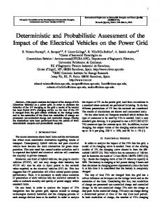
hence, the criterion for the multidimensional problem is a generalization of that used in the onedimensional case. • d(f, fˆ) is calculated through a Monte Carlo method which involves the concept of Voronoi partitions. • The procedure consists in searching for ! the discre" ˆ that minimizes E |X − X| ˆ ; the te random vector X ˆ and the correpossible values x(1), . . . , x(N ) of X sponding weights w(1), . . . , w(N ) generate the discrete approximation fˆ of the density f .
6
M odel ϕ
0.2
D( 0.7 m)
1.2
0.5
5 w H2
9.5 %) O(
x(5)
6.5 ! 7" log10 m(kg/s) ˙
7.5
MC SQ, NSQ = 20 SQ, NSQ = 15 SQ, NSQ = 10
6
6.5 ! 7" log10 m(kg/s) ˙
7.5
variable X1 ˆ x(1) , . . . , x(7) → possible values of X
• It can be shown that, in the case d = 1, !
Figure 5: the correspondence between the distribution of mass flow rate found with 1000 MC simulations and SQ method is fully satisfactory when NSQ = 20.
5 (%) O w H2
MC
quantization
Stochastic
E w2
M odel
D( 0.7 m)
• One-dimensional steady model of magma flow in a cilindrical conduit with fixed diameter and uniform temperature [1].
that minimize the quantity d(f, fˆ).
"
6
variable X
• When X is a d-dimensional vector quantity, a different definition of distance is more appropriate.
output discretization N = 10
Figure 4: with the SQ method and only N = 20 simulations, we approximate the true values at a confidence level corresponding to N = 2000 MC simulations for the mean or N = 200 MC simulations for the standard deviation.
w2
• The procedure consists in searching for N points !
50 100 200 500 1000 2000 numerosity
Fˆ (x)
1
ˆ be a discrete random vector with probability • Let X distribution fˆ, approximating a continuous random vector X. The distance between f and! fˆ can! be ! ˆ !! redefined as the mean value of the error !X − X ˆ We thus sulting from the substitution of X with X. minimize
M odel
discrete
The multi-parameter input case, d>1 variable Y
N = 10
cumulative
F (x)
distribution
quantization
input discretization
countinuous
20
ϕ(X1, X2) = X12X22.
w10
output
variable X1
• there is a maximum number N of affordable simulations.
• find N values of X,
M odel
1
variable X2
input
100 200 500 1000 2000 numerosity
• The case in the figure refers to
unknown
probability density
known
probability density
• the random vector X = (X1, . . . , Xd) is part of the input data of a numerical code ϕ and the random variable Y is one relevant model output;
probability density
A practical situation:
2
50
3
(1)
where xmin and xmax are the minimum and maximum possible values of X.
and N corresponding weights
What is stochastic quantization?
20
Figure 3: implementation of the multi-parameter input case. The blue points are a sample of X = (X1, X2); the ˆ orange points x(1), . . . , x(7) are the possible values of X, which is a discrete approximation of X. The orange lines define the Voronoi regions generated by the set of points x(1), . . . , x(7): the region associated to x(i) contains the blue points which are closer to x(i) than to any other of the orange points.
CONCLUSIONS The SQ method allows the introduction of uncertainties in the deterministic approach without requiring exceeding CPU time. As a consequence, volcanic scenarios can be estimated in the future by means of complex deterministic models and taking into account the intrinsic uncertainties involved in the definition of volcanic systems.
This poster participates in
References [1] P. Papale, Dynamics of magma flow in volcanic conduits with variable fragmentation efficiency and nonequilibrium pumice degassing, J. Geophys. Res., 106, 11043-11065, 2001 [2] S. Graf, H. Luschgy, Foundations of quantization for probability distributions, Springer-Verlag, 2000
YSOPP
G
en
9
• We are therefore developing the application of stochastic methods to largely reduce the computational costs.
50 100 200 500 1000 2000 numerosity
0.16
probability distribution
• Taking into account these uncertainties in predictive models can be exceedingly demanding.
20
0.05
probability distribution
• Some of the quantities which determine volcanic processes are uncertain.
0.2
0.18
probability density
• Volcanic systems are largely out of direct observation.
1
variable X2
We present the stochastic quantization (SQ) method for the approximation of a continuous probability density function with a discrete one. This technique reduces the number of numerical simulations required to get a reasonably complete picture of the possible eruptive conditions at a considered volcano. Finally we show the results of a test using a one-dimensional steady model of magma flow [1] as a benchmark.
• Introduce a distance between two probability distributions, in the case in which X is a scalar quantity: if F (x) is the cumulative distribution function associated with the density f (x) and Fˆ(x) is the one associated with its discretization fˆ(x), we define the distance between f and fˆ as follows:
probability
• The demand for eruption scenario forecast is pressing.
The single parameter input case, d=1
probability
Abstract
1
0.22
0.055
• Let ϕ(X) be a known analytical function. The probability distribution of the output random variable Y can be calculated exactly and compared with the approximations produced by SQ and by Monte Carlo (MC) methods with variable numerosity.
probability
Rationale
MC real value SQ, N = 20
0.06
Istituto Nazionale di Geofisica e Vulcanologia, Sezione di Pisa, Italy 3
MC real value SQ, N = 20
0.07
probability density
2
Normale Superiore, Pisa, Italy
0.24
0.075
0.105
0.1
1 Scuola
0.26
0.08
mean
E. Peruzzo1, L. Bisconti2, M. Barsanti2,3, F. Flandoli3 and P. Papale2
5
era
l A s s e m b ly
20
0
Young Scientists' Outstanding Poster Paper Contest