to the behavior of the key quality characteristics. When deal- ing with continuous characteristics, the Gauge R&R is regarded as the statistical technique in MSA.
Quality Engineering, 17:495–507, 2005 Copyright # Taylor & Francis Inc. ISSN: 0898-2112 print=1532-4222 online DOI: 10.1080/08982110500225562
A Comparison of Methods for the Evaluation of Binary Measurement Systems Wessel N. van Wieringen† and Edwin R. van den Heuvel§ Institute for Business and Industrial Statistics of the University of Amsterdam, Amsterdam, The Netherlands
Many quality programs prescribe a measurement system analysis (MSA) to be performed on the key quality characteristics. This guarantees the reliability of the acquired data, which serve as the basis for drawing conclusions with respect to the behavior of the key quality characteristics. When dealing with continuous characteristics, the Gauge R&R is regarded as the statistical technique in MSA. For binary characteristics, no such universally accepted equivalent is available. We discuss methods that could serve as an MSA for binary data. We argue that a latent class model is the most promising candidate. Keywords
Kappa; Intraclass correlation coefficient; Latent class model; Log-linear model; Measurement system analysis.
INTRODUCTION It may happen that the quality of a part does not meet a desired level. The improvement of the quality of such a part is achieved by following the method of empirical research. Keystone to this method is the collection of measurements on which conclusions are based. Thus, the measurements are guiding in how to improve the quality. The quality of the measurements determines the usefulness of the measurements to empirical investigation. The quality of measurements is directly related to the uncertainty of measurement. The uncertainty of measurement (and y
Current affiliation: Department of Statistics, Free University of Amsterdam. x Current affiliation: Organon NV. Address correspondence to Wessel N. van Wieringen, Eikenweg 24, 1092 CA, Amsterdam, The Netherlands. Note: The following is the address for the Institute for Business and Industrial Statistics of the University of Amsterdam, where all the work in relation to the article was carried out, Plantage Muidergracht 24, 1018 TV Amsterdam, The Netherlands.
consequently the quality of measurement) is assessed through a measurement system analysis (MSA) study. An MSA study prescribes an experiment that is designed to allow for the assessment of the uncertainty of measurement. Traditionally (Wheeler and Lyday, 1989), an experiment for the evaluation of a measurement system is designed such that n parts are being judged by m raters, preferably repetitively, say l times. When dealing with continuous measurements, it is assumed that the outcome of the experiment can be modeled by a two-way, random-effects model. Let Xijk the kth judgment of operator j on part i, the model then is Xijk ¼ l þ ai þ bj þ cij þ eijk ;
ð1Þ
where l is the overall mean common to all observations, ai � Nð0; r2a Þ; bi � Nð0; r2b Þ, cij � Nð0; r2c Þ and eijk � Nð0; r2e Þ, and the random variables are independent for i ¼ 1; . . . ; n; j ¼ 1; . . . ; m and k ¼ 1; . . . ; l. Then, the variance component r2b þ r2ab þ r2e is the operationalization of the uncertainty of measurement. It provides the information needed to construct a confidence interval for the true value of a part’s quality. However, in practice, one often encounters measurement systems that are noncontinuous; for instance, a quality characteristic that only assumes two values, a so-called binary measurement. In an industrial setting, such a situation may arise when quality of a part is evaluated through visual inspection, resulting in parts labeled either defective or nondefective. Assuming the aforementioned experimental design is also the most sensible for binary measurements, it is not clear how the outcome of the experiment should be modeled. Moreover, this model should give rise to an operational definition of the uncertainty of measurement in the binary context. In this article, we model the outcome of an MSA experiment of binary measurement system by means of a latent class model (in line with Boyles, 2001). Within this latent class model, we give an operational
495
496
W. N. van Wieringen and E. R. van den Heuvel
definition of uncertainty of measurement. Next, we compare the latent class model with alternative approaches1 that are currently used to evaluate the measurement system, namely the kappa statistic, the intraclass correlation coefficient, and log-linear models. This comparison shows the best way to analyze an MSA study for binary measurements. We conclude with a case study that illustrates all techniques discussed. LATENT CLASS MODEL Consider an MSA experimental design as described in the introduction, where n parts are being judged by m raters only once (for the purpose of comparing several techniques, it is most illustrative to disregard repetitions). Ideally, the sample of parts involved is a good representation of the parts one expects to encounter in later investigations. So far, we do not know the quality of measurements. Therefore, theoretically, we have no information of the true state, henceforth called Y , of any part. As parts are selected randomly, we regard Y as a random variable, taken to be Bernoulli distributed with unknown parameter h ¼ PðY ¼ 1Þ, the probability of the part being of good quality. Let a sample of m raters be involved in the MSA experiment. Associated with each rater, we define a random variable Xj ðY Þ, the judgment of rater j, which depends on Y , the true state of the judged part. Xm is also Bernoulli distributed, with parameter pj ðyÞ ¼ PðXj ¼ 1jY ¼ yÞ, where we have dropped (for notational convenience) the argument Y in Xj ðY Þ. The unconditional probability that a randomly selected part is judged as xj 2 f0; 1g by rater j is then given by pj ðxj Þ ¼ PðXj ¼ xj Þ
PðX1 ; X2 ; . . . ; Xm jY Þ ¼
m Y
PðXj jY Þ;
ð3Þ
j¼1
(i.e., given the true state of the part, the raters judge independently). Because both the observed and latent variable are Bernoulli, the unconditional probability that rater j judges a part as good can be written as in Eq. 2. Using this and Eq. 3, we can specify the model underlying the latent class analysis. Hereto, let X denote the n � m matrix, containing the data from the MSA experiment, with Xij the judgment of rater j on part i, given by: 0 1 X11 . . . X1m B . .. C .. X ¼ @ .. . A . Xn1
. . . Xnm
We repeat that, for illustration purposes, we assume the operators to judge each part only once. However, the method described here is naturally extended to the situation where multiple judgments are made by each operator, as one expects in a regular MSA experiment for continuous measurements. Then, the likelihood function of the joint response of the raters of the sample, X, becomes LðX; h; p1 ð1Þ; . . . ; pm ð0ÞÞ ¼
n Y
ð1 � hÞ
i¼1
m � Y
pj ð0Þ
�Xij �
1 � pj ð0Þ
�1�Xij
j¼1
þh
m � Y
! �Xij � �1�Xij pj ð1Þ 1 � pj ð1Þ ;
ð4Þ
j¼1
¼ PðXj ¼ xj jY ¼ 0ÞPðY ¼ 0Þ þ PðXj ¼ xj jY ¼ 1ÞPðY ¼ 1Þ
that it assumes conditional independence. That is, given the realization of the latent variable, the manifest variables are independent of one another. Conditional independence can be formulated as
ð2Þ
Latent class analysis distinguishes between a manifest variable (the judgment of a rater) and an unobserved, latent variable (the true value of the part). The latter is used to explain the correlated structure in the (observed) former. Crucial to this approach is
where we substituted PðY ¼ 1Þ ¼ h and PðXij ¼ 1jY ¼ yÞ ¼ pj ðyÞ for all j and y. In addition, we impose restrictions on the model to ensure identification because this is not automatically guaranteed. To see this, choose any vector of parameters W0 ¼ ðh0 ; p01 ð1Þ; . . . ; p0m ð1Þ; p01 ð0Þ; . . . ; p0m ð0ÞÞT , and define W� ¼ ð1 � h0 ; p01 ð0Þ; . . . ; p0m ð0Þ; p01 ð1Þ; . . . ; p0m ð1ÞÞT : ð5Þ
1
We realize that the automotive industry (Automotive Industry Action Group, 2002) has prescribed a way to conduct an attribute gauge study. It assumes the qualitative evaluation of a part can be compared with an underlying continuous measurement. However, as knowledge of this continuous measurement is not always at hand, we disregard it here.
Then, for any response pattern, due to symmetry in the density function: PðX ¼ x; W0 Þ ¼ PðX ¼ x; W� Þ:
497
Comparison of Methods for Evaluation of Binary Measurement Systems
Therefore2 in the particular case where each operator makes only one judgment, we need to involve at least three operators and require that h 2 ð0; 1Þ and 1 � pj ð1Þ > pj ð0Þ � 0 for all j. The restriction pj ð1Þ > pj ð0Þ follows naturally because it merely states that the probability of operator m judging a good part as such is higher than the probability that he judges a bad part as good. Now, Eq. (4) plus these restrictions enable one to use a maximum likelihood procedure to estimate all parameters, confer Bartholomew and Knott (1999) and Boyles (2001). To find a maximum likelihood estimate for W, instead of applying the traditional Newton-Raphson algorithm, the so-called E-M algorithm is used (see the Appendix). It has been shown that the sequence of estimates produced by the E-M algorithm converges to a maximum of the likelihood function, confer McLachlan and Krishnan (1997).
system (i.e., the number of parts judged wrongly). Its importance is eminent in the context of acceptance sampling on attributes when meeting requirements as AQL, LQL, AOQL, etc. Also, in the context of quality improvement knowledge of the probability of misclassification is of importance when it comes to drawing conclusions with respect to key factors influencing the key quality characteristic. Once the parameters p1 ð0Þ; . . . ; pm ð0Þ and p1 ð1Þ; . . . ; pm ð1Þ have been estimated, it is straightforward to calculate the probability of misclassification. Assuming, for simplicity (other distributions only ask for small changes), that during regular production all raters judge an equal share of the parts, then, for any quality h of the sample, the probability of misclassification is Pðincorrect decisionÞ ¼
OPERATIONAL DEFINITION The latent class approach also allows for a natural operationalization of the uncertainty of measurement. The uncertainty of measurement of binary measurements is that of misclassification. That is, a part may have been measured as belonging to one category, although in fact it originates from its complement. For instance, a defective part that has been, for whatever reason, measured as a nondefective, or vice versa. Therefore, we propose—for binary measurement systems—an operational definition of the uncertainty of measurement to be related to the probability of misclassification. However, the probability of misclassification itself depends on the sample one studies, whereas preferably the evaluation of the measurement system is independent of the sample. Compare the continuous case where the variance component (which is the operationalization of uncertainty of measurement there) is independent of the mean and variation of the parts in the sample. Therefore, we adopt from Uebersax (1988) the terms sensitivity defined as the probability that a good part is rated as such, and specificity as the probability that a bad part is rated as bad. These definitions coincide with the indices pj ð1Þ and 1 � pj ð0Þ. This operational definition allow us, given the quality of the sample, to calculate the probability of misclassification. Thus, giving a clear insight into the consequences of this measurement
2
The proof of these restrictions is beyond the scope of this article.
m � 1X hð1 � pj ð1ÞÞ m j¼1 � þð1 � hÞpj ð0Þ :
ð6Þ
In addition, on the individual part level, one can indicate which category the part most likely originates from. That is category y that maximizes: PðY ¼ yjXi1 ; Xi2 ; : . . . ; Xim Þ. Besides these favorable features of the latent class model, it has two main drawbacks. It requires many measurements to give an accurate estimation of the parameters. However, this is inherent to binary data. Second, for the estimation of the parameters an algorithm is needed (hardly a problem in the present computer age).
ALTERNATIVE METHODS Measure of Agreement An alternative to the latent class model is Cohen’s kappa (Cohen, 1960). This statistic has been proposed as a useful statistic for the evaluation of categorical measurement systems, confer Boyles (2001), Futrell (1995), and Dunn (1989). Recently, the statistical software package Minitab reports the kappa in its Attribute Gauge R&R study for the evaluation of the measurement system. Many measures representing the quality of the measurement system have been proposed, confer Goodman and Kruskal (1954) and the review papers of Landis and Koch (1975a) and (1975b). Cohen (1960) introduced a measure of agreement called the kappa. There is agreement if two measurements (on the same part) are equal. The kappa represents the
498
W. N. van Wieringen and E. R. van den Heuvel
degree of agreement between two raters, based on how they classify a sample of parts into a number of categories. Cohen’s observed agreement may be due to chance. Hence, Cohen defined the kappa, denoted j, corrected for agreement by chance and normalized, as j¼
Po � Pe : 1 � Pe
ð7Þ
Here, Po is the observed proportion of agreement and Pe the expected proportion of agreement due to chance. Kappa attains the value one when there is perfect agreement, zero if all observed agreement is merely due to chance, and negative values when the amount of agreement is less, then is to be expected on the basis of chance. Often, the observed proportion is used to evaluate the judgment process. However, Po � j, and thus Po , always gives a better impression of the measurement system than when chance, agreement is taken into account. As a comparison, consider an exam with only multiple-choice questions. Its grades are calculated in accordance with Eq. 7. That is, the proportion of questions the examinee answered correctly, Po , is lessened by the expected proportion of questions he got right had he chosen his answers randomly, Pe . This difference is scaled such that grades fall in the aimed range. Cohen (1960) specified, for any pair of raters j1 and j2 , the terms in Eq. 7 as Po ¼
1 X x¼0
pj1 ;j2 ðx; xÞ
and
Pe ¼
1 X
pj1 ðxÞ pj2 ðxÞ:
x¼0
Here, Po is the proportion of parts with matched judgments of raters j1 and j2 and pj1 ; j2 ðx; xÞ denoted the proportion parts that have been judged as x by raters j1 and j2 . Pe is the expected proportion of agreement based on the individual marginal distributions of each rater. The marginal proportion for rater j and category x is denoted by pj ðxÞ. Due to the way Pe is calculated, j may give values that are counterintuitive. For instance, suppose that all raters measure most parts in the same category (small part variation). Then, j is small, as Pe is large. Thus, j confounds to some extent uncertainty of measurement of the measurement system with part variation. Similarly, let one rater measure almost all parts in one category, and the other rater almost all of them in a different category (systematic rater difference). Then, Pe approaches its minimum and causes a relatively high j. Thus, whereas j is designed to measure systematic rater differences, it ignores them to some extent. These are called the paradoxes of the
kappa, confer Cicchetti and Feinstein (1990) and Feinstein and Cicchetti (1990). In this context, it has been argued (Brennan and Prediger, 1981) to define agreement by chance as completely random (i.e., the raters assign the parts to any category with equal probability). Thus, in line with a contingency table setting, Cohen assumes an independence model based on the individual marginal proportions. He then constructs a sample statistic, j, of which he claims measures the degree of agreement between the raters. As suggested by Futrell (1995) and Dunn (1989), this statistic can be used to evaluate the quality of measurements. However, the relation between degree of agreement and uncertainty of measurement has never been specified. This, together with j’s paradoxes, makes it unsuitable for the evaluation of the quality of measurements. If one uses the j method, the following criteria can be applied that apparently guarantee a reliable measurement system. Landis and Koch (1977) give a table (see Table 1) that expresses the relationship between the value of j and the corresponding evaluation of the measurement system. Although as they suggest themselves, their classification is rather arbitrary. Another approach is to test H0 : j ¼ 0 against HA : j 6¼ 0, thus testing whether agreement is substantial, or merely due to chance. For more on test procedures and moments of the j, check Everitt (1968) and Hubert (1977).
KAPPA FOR MULTIPLE RATERS It is not straightforward to extend the kappa statistic to more than two raters case. We point out shortly how this is done. Because at least two people are necessary for agreement, Fleiss (1971) suggested the degree of agreement may be expressed in terms of the proportion of agreeing pairs. If there are m raters, then the maximum possible number of agreeing pairs per part equals 12 mðm � 1Þ. To estimate the proportion of agreeing pairs per part, Fleiss (1971) proposed the sum of the number of agreeing pairs per category. Then, to get an overall estimate for the observed proportion of agreement, we take the sum over the parts of all these proportions, scaled with the total number of possible agreeing pairs. In formula ! n X 1 X 1 Po ¼ ni ðxÞðni ðxÞ � 1Þ ; nmðm � 1Þ i¼1 x¼0 with ni ðxÞ the number of times part i has been classified as x. The expected proportion of agreement is
Comparison of Methods for Evaluation of Binary Measurement Systems
given by Pe ¼
m X 1 X 2 pj ðxÞpj2 ðxÞ: mðm � 1Þ j1 ; j2 ¼1 x¼0 1 j1 < j2
It should be clear that each pair of raters enters the sum only once. Pe estimates, under the assumption of independence, the probability that two randomly selected raters classify a part into the same category, based on the individual marginal proportions of the raters. Note that we have adopted Conger (1980) here instead of Fleiss (1971). The main difference with Fleiss (1971) is that Conger (1980) allows the raters to have different marginal distributions and calculates Pe without rater replacement. This has the advantage that it is conceptually in line with Cohen (1960). This is illustrated by the fact that it equals the average of all Cohen’s (1960) pairwise kappa’s, if either there is independence between all raters or their marginal probabilities are equal. One may generalize this by looking at other tuples of agreeing raters. KAPPA STATISTIC VERSUS LATENT CLASS MODEL The latent class model is a model for the outcome of an MSA experiment, whereas j is merely a sample statistic.Using the latent class model, we can rewrite j in terms of the parameters of the latent class model. We limit ourselves to two raters3, mainly to avoid cumbersome notational issues. Then, the observed agreement is the probability that both raters make the same judgment: Po ¼ PðX1 ¼ X2 Þ 1 X
¼
j1 � y � hjðx � p1 ðyÞÞðx � p2 ðyÞÞ
x;y¼0
and the expected proportion of agreement (i.e., the probability that by chance the raters judge similarly), which is given by Pe ¼
1 X x¼0
PðX1 ¼ xÞPðX2 ¼ xÞ ¼
1 X
p1 ðxÞp2 ðxÞ;
x¼0
with pj ðxÞ given by Eq. (2). It should now be clear how to reformulate Eq. (7) in terms of the latent class parameters. This yields a j that depends on the pj ðyÞ and on the process parameter h. We have displayed 3
This violates the identification restrictions but can be coped with by in addition requiring that pj ð0Þ ¼ 1 � pj ð1Þ for j ¼ 1; . . . ; m.
499
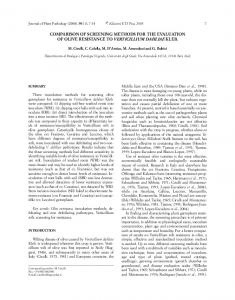
this graphically, for an arbitrary choice of the pj ðyÞ, by plotting j against h, see Figure 1. Thus, for one and the same measurement system j can differ substantially from one MSA experiment to another depending on the quality of the sample involved. This may result in an evaluation of the measurement system that is at odds with evaluations based on MSA experiments involving other samples. Given the fact that kappa depends on the process parameter h, one may argue that the criteria on the kappa, as proposed in Landis and Koch (1977), should be adjusted accordingly, confer Elffers (2001). It remains unclear how this should be done. Moreover, because the criteria themselves are arbitrary, so will their adjustments be. The latent class model is a model for the outcome of the MSA experiment, whereas kappa is merely a summary statistic, trying to summarize all aspects of a measurement system into one number, an almost impossible task. Moreover, when it indicates that the measurement system is not up to standard, it provides no clues as to how this has arisen. The latent class model yields information about the individual rater performances, thus given insight how discrepancies between judgments come about. INTRACLASS CORRELATION COEFFICIENT For continuous measurement systems, the intraclass correlation coefficient is often used to assess the uncertainty of measurement (Shrout and Fleiss, 1979). The intraclass correlation coefficient measures the correlation among multiple measurements of the same part. The intraclass correlation coefficient can also be used to evaluate the uncertainty of measurement of binary measurement systems. For binary measurements, the intraclass correlation coefficient is called the / coefficient and (for two raters) defined as CovðXi1 ; Xi2 Þ / ¼ pffiffiffiffiffiffiffiffiffiffiffiffiffiffiffiffiffiffiffiffiffiffiffiffiffiffiffiffiffiffiffiffiffiffiffiffiffiffiffi VarðXi1 Þ � VarðXi2 Þ PðXi1 ¼ 1; Xi2 ¼ 1Þ � p1 p2 ¼ pffiffiffiffiffiffiffiffiffiffiffiffiffiffiffiffiffiffiffiffiffiffiffiffiffiffiffiffiffiffiffiffiffiffiffiffiffiffiffiffiffiffiffiffi : p1 ð1 � p1 Þ p2 ð1 � p2 Þ
ð8Þ
As other product moment correlation coefficients / only assumes values in the interval [�1,1]. The / coefficient is estimated by replacing all the terms in the righthand side ofP Eq. 9 by p2 ¼ their p1 ¼ 1n Pni¼1 Xi1 ; b Pn corresponding estimates: b n 1 1 X , and PðX ¼ 1; X ¼ 1Þ by X X i2 i1 i2 i1 i2 : i¼1 i¼1 n n For the situation involving m > 2 raters, Fleiss (1965) and Bartko and Carpenter (1976) propose to
500
W. N. van Wieringen and E. R. van den Heuvel
Figure 1.
evaluate the reliability by means of the average of the / coefficients of all possible rater pairs, where they assume that pj ¼ p for j ¼ 1; . . . ; m. The / coefficient for multiple raters is then estimated by / ¼ ðP � p2 Þ= ðp � p2 Þ, where n X m 1 X Xij P¼ nm i¼1 j¼1 and n m �1 X m X X 2 P¼ Xij Xij nm ðm � 1Þ i¼1 j ¼1 j ¼j þ1 1 2 1
2
1
When using / as the statistic representing the quality of measurements, from Wheeler and Lyday (1989) one can distract the following criteria for / (Table 2). The criteria in Table 2 apply to intraclass correlation coefficients for continuous measurements. We assume they can be used for / coefficient.
j against h.
INTRACLASS CORRELATION COEFFICIENT VERSUS LATENT CLASS MODEL As with the kappa statistic, we use the latent class model to study the intraclass correlation coefficient and restrict ourselves to the two rater case. To this extent, the numerator of / becomes CovðXi1 ; Xi2 Þ ¼
1 X
ðx1 � p1 ð1ÞÞðx2 � p2 ð1ÞÞ
x1 ;x2 ¼0
� PðX1 ¼ x1 ; X2 ¼ x2 Þ ¼ h ð1 � hÞ ðp1 ð1Þ � p1 ð0ÞÞ ðp2 ð1Þ � p2 ð0ÞÞ; and its denominator is
pffiffiffiffiffiffiffiffiffiffiffiffiffiffiffiffiffiffiffiffiffiffiffiffiffiffiffiffiffiffiffiffiffiffiffiffiffiffiffi VarðXi1 Þ � VarðXi2 Þ, where
501
Comparison of Methods for Evaluation of Binary Measurement Systems Table 1 Correspondence between j and the quality of measurements j