A Scout robot with an upward-facing Omnitech 190⦠fisheye lens. The lens provides 360⦠horizontal field of view around the robot, effectively functioning as an ...
A Comparison of Maximum Likelihood Methods for Appearance-Based Minimalistic SLAM Paul E. Rybski, Stergios I. Roumeliotis, Maria Gini, Nikolaos Papanikolopoulos Center for Distributed Robotics, Department of Computer Science and Engineering University of Minnesota, Minneapolis, MN, 55455 Email: {rybski,stergios,gini,npapas}@cs.umn.edu
Abstract— This paper compares the performances of several algorithms that address the problem of Simultaneous Localization and Mapping (SLAM) for the case of very small, resource-limited robots. These robots have poor odometry and can typically only carry a single monocular camera. These algorithms do not make the typical SLAM assumption that metric distance/bearing information to landmarks is available. Instead, the robot registers a distinctive sensor “signature”, based on its current location, which is used to match robot positions. The performances of a physics-inspired maximum likelihood (ML) estimator, the Iterated form of the Extended Kalman Filter (IEKF), and a batch-processed linearized ML estimator are compared under various odometric noise models.
I. I NTRODUCTION Spatial reasoning algorithms used for solving the Simultaneous Localization and Mapping (SLAM) problem for mobile robots typically require the use of fairly good odometric estimates and/or accurate range sensors. Very small robots such as the Minnesota Scout [1], shown in Figure 1, have very restricted sensing and very poor odometry. The Scout only has a single monocular camera whose video must be broadcast to a nearby workstation for processing. Robot control is achieved with a wireless proxy-processing scheme whereby the decision processes are run on the workstation.
In previous work, we proposed a modification to the standard SLAM algorithm in which we relax the assumption that the robots can obtain metric distance and/or bearing information to landmarks. In this approach, we obtain purely qualitative measurements of landmarks where a location “signature” is used to match robot pose locations. In this method, landmarks correspond to sensor readings taken at various (x, y) positions along the path of the robot. This is a divergence from most SLAM approaches where landmarks represent specific objects of a known type in the environment such as edges, corners, and doors. We hereafter compare and contrast previously proposed solutions to this problem that involved a heuristic physics-inspired maximum likelihood (ML) method [2], as well as an Iterated Extended Kalman Filter (IEKF) method [3]. In this paper, we propose a batch-processed linearized ML algorithm which addresses some of the shortcomings of the previously proposed physics-based and Extended Kalman filter models. Unlike the physics-based heuristic method, the proposed method explicitly reasons about the uncertainty in the sensor readings and determines the most likely path of the robot using all of the available sensor data at the end of a lengthy and circuitous path. Additionally, this method iterates over all of the robot’s data at once rather than in an on-line fashion like the IEKF. This tends to produce robust estimates as it is capable of handling the nonlinearities in the system in an iterative and more robust fashion. Experimental results are described which show that this method produces more accurate position estimates than either of the two proposed methods for this problem. II. R ELATED W ORK
Fig. 1. A Scout robot with an upward-facing Omnitech 190◦ fisheye lens. The lens provides 360◦ horizontal field of view around the robot, effectively functioning as an omnicamera. The robot is 11 cm long and 4 cm in diameter.
Physics-based ML estimators that involve spring dynamics have been used quite effectively to find minimum energy states in metric/topological map structures [4] as well as relative robot poses [5]. The Extended Kalman Filter has been used for localizing [6] and performing SLAM [7] on mobile robots for at least a decade. Our approach differs from these estimators in that we do not have the ability of resolving specific geometric information about the landmarks the robot observes in its environment. Instead, landmark positions are explicitly coupled to the position of the robot. Bayesian methods have also been used for mobile robot localization and mapping [8] where the modes of arbitrary
robot pose distributions are computed. Statistical methods such as Monte Carlo localization [9] use sampling techniques to estimate arbitrary distributions of robot poses. These methods typically use very accurate sensors and/or robots with accurate odometry to resolve maps over large distances. In previous implementations of SLAM algorithms, it is frequently assumed that the robot is able to measure its relative position with respect to features/landmarks [10], [11] or obstacles [8] in the area that it navigates. This implies that the robot carries a distance measuring sensor such as a sonar or a laser scanner. The algorithms described in this work are designed for robots that have no such sensor modality. Structure from motion (SFM) [12] algorithms compute the correspondences between features extracted from multiple images to estimate the geometric shape of landmarks as well as to estimate the robot’s pose. Sim and Dudek [13] describe a visual localization and mapping algorithm which uses visual features to estimate the sensor readings from novel positions in the environment. In practice, our vision system could be replaced by any other kind of boolean sensor modality which can report whether the robot has re-visited a location. An alternative approach is to use a small camera and process relative angular measurements to detected vertical line features, as described in [14]. However the applicability of this algorithm is conditioned on the existence of a sufficient number of identifiable vertical line segments along the trajectory of the robot. Also it is geared toward position tracking while no attempt is made to construct a map populated by these features. In contrast to explicit metric-based methods, more qualitative methods such as topological maps of nodes, such as Ben Kuipers’ Semantic Spatial Hierarchy (SSH) [15], have been suggested. Locations are explicitly designated by distinctive (but not necessarily unique) sensor signatures. In [16], image “signatures” captured from an omnidirectional camera are used to construct a topological map of an environment by generating histograms of the RGB and HSV (Hue, Saturation, and Value) components. III. A PPEARANCE -BASED M APPING FOR S MALL ROBOTS Mobile robots such as the Scouts are able to track their pose for a limited amount of time by integrating kinetic information from their wheel encoders. Without any sort of absolute position measurement from another sensor, the noise in the velocity measurements will eventually cause the computed pose estimates to diverge wildly from their real values. In order to provide periodic corrections, additional information is necessary. In environments where GPS measurements are not available, a robot will have to use information about its surroundings for this purpose. In what follows, we describe and implement a novel methodology that neither relies on any specific type of visual features, nor requires distance measurements. This concept is illustrated in Figure 2. The basic idea behind our approach is to determine a unique visual signature for distinct locations along the robot’s path, store this and the estimated pose of the robot at that time instant, and retrieve this information
once the robot revisits the same area. Determining whether the robot is at a certain location for a second time is the key element for providing positioning updates. By correlating any two scenes, we infer a relative (landmark to robot, not landmark to landmark) position measurement and use it to update both the current and previous (at locations visited in the past) pose estimates for the robot. This in effect will produce an accurate map of distinct locations within the area that the robot has explored.
Fig. 2. Appearance-based mapping. Virtual sensor “signatures” are used to identify specific (x, y) locations in space. The sensors are assumed not to return any spatial information about the environment.
IV. T HE BATCH M AXIMUM L IKELIHOOD E STIMATOR In our previous work, a physics-inspired ML estimator was derived which used numerical simulation to find the most likely map given a highly non-linear system. However, this estimator made several significant assumptions about the problem. First, it was assumed that when the robot crossed its own path, the nodes would occupy the same physical location in space. Secondly, it was assumed that the linear and torsional motion estimates could be treated separately. While these assumptions might not reduce the quality of the estimates such that they are unusable, they will produce an estimate that is not as accurate as it could be. In order to incorporate this information, the estimator’s cost function needs to be formulated in a different way. A. Motion and Sensor Models In this new formulation, the robot’s proprioceptive estimate of how far it traveled between one location and another is the same as in the previous estimator. This is computed by integrating a series of readings from the robot’s odometric sensors (wheel encoders) to determine the relative displacement (x, y, θ). The cost function for this estimate is called the motion cost function and is described as: (yi − hyi (X))T Pi−1 (yi − hyi (X))
(1)
where yi is a vector that describes the measured displacement between the previous position measured at time i−1 and the current position measured at time i. The function hyi (X) computes the predicted displacement of the robot given the current state vector from time i − 1 to time i. The covariance
of this measurement is Pi , which represents the uncertainty in the robot’s pose. The state vector of a ML estimator consists of the necessary parameters to solve for. For the case of a mobile robot moving on a 2D surface, the variables represent individual locations to which the robot has traveled. If the robot returns to a location that it has already visited, it is often assumed that those two locations are identical. However, this assumption is not quite true since while the robot may have traveled near the same location several times, those exact positions of the robot are not completely identical. This means that simply merging the nodes will not provide the most accurate estimate. To correct this, a sensor cost function must be defined and integrated into the equation: (zi − hzi (X))T Ri−1 (zi − hzi (X))
(2)
In this sensor cost function, zi is a vector that describes the measured displacement between a position measured previously at time j (not limited to time i − 1) and the current position at time i. Using the notion of the appearance-based sensor, the value of zi will always be 0 since the landmarks correspond directly to the positions of the robot. The function hzi (X) computes the predicted displacement of the robot given the current state vector from the previously-seen location at time j to the current time i. The covariance of this measurement is Ri , which represents the accuracy of the place recognition sensor, or a region around a specific location where the location appears to be the same. As the robot discovers new landmarks (a sensor reading that the robot has seen before), it augments the state vector with their positions and marks those variables as the locations of the original sightings. The sensor cost function in Equation 2 always compares the current measured position of a landmark against the first discovered position of that landmark. Combining the motion and sensor cost functions (Equations 1 and 2), the complete cost function is: X
(yi − hyi (X))T Pi−1 (yi − hyi (X)) +
i
X
(zj − hzj (X))T Rj−1 (zj − hzj (X))
(3)
j
The number of motion cost function terms is the number of sensor readings minus one |S| − 1. The number of sensor cost function terms corresponds to the number of non-unique landmarks the robot has identified. B. Iterative State Update The non-linear nature of this problem, introduced by the need to handle the rotational component of the robot, means that finding the best solution can be analytically and computationally challenging. In our previous work, with a the spring and mass-based estimator, a numerical solution was determined for computing the minimum for finding the minimum value of the cost function. A more analytical method for
finding the minimum solution is to linearize the system with a first-order linear approximation such as a Taylor series expansion. Thus, the sensor and motion measurement functions take the form: ˆ + ∇X h(X) h(X) ≈ h(X)
ˆ X=X
ˆ (X − X)
ˆ + H(X − X) ˆ ≈ h(X)
(4)
ˆ is the where X is the true (unknown) state vector and X robot’s estimate of the state vector. Expanding this equation for each of the cost functions and taking the first derivative to solve for its minimum, a recursive formulation of the estimator can be obtained. Applying the first-order Taylor expansion to the cost functions obtains an expression of the form: n−1 X
`
yi − hyi (X)
i=1 n X
`
´T
zi − hzi (X)
−1
Pi
´T
`
−1
Ri
´ yi − hyi (X) + `
´ zi − hzi (X) ≈
i=1 n−1 X“
ˆ yi − hyi (X) − Hyi (X − X)
i=1 n “ X
”T
ˆ zi − hzi (X) − Hzi (X − X)
−1
Pi
”T
“ ” ˆ + yi − hyi (X) − Hyi (X − X)
−1
Ri
“
ˆ zi − hzi (X) − Hzi (X − X)
”
i=1
(5)
This function is quadratic in X. To minimize the function with respect to X, the first derivative is taken and the equations are set to 0. This results in an equation with the following form: ˆ+ X=X
n−1 X i=1
HyTi Pi−1 Hyi
+
n X
!−1 HzTi Ri−1 Hzi
i=1
n−1 X
! n “ ” “ ” X −1 −1 ˆ ˆ Hzi Ri zi − hzi (X) yi − hyi (X) + Hyi Pi
i=1
i=1
(6)
where the X on the right-hand side of the equation is the initial estimate of the system. The first value of this estimate can be obtained from the robot’s raw odometry, if no other estimate is available. This is a recursive form where the result from the left-hand side of the equation is plugged back into the equation on the right-hand side. This first-order linear approximation of the measurement function is only valid for small errors in the estimate of X. As the equations are iterated, the state estimate should converge to a final solution. The above defines the recursive form for the ML estimator. Now, the expressions for the individual sensor measurements (odometry propagation and virtual place sensor) must be defined. C. Odometry Propagation Measurement The measurement function for the distance estimates between subsequent nodes based on their odometry is defined as:
V. V ISION -BASED F EATURES T hyi (X) = R G C (φR ) XLi − XLi−1
�
T
(7) T
where XLi = [xi yi φi ] and XLi−1 = [xi−1 yi−1 φi−1 ] are the positions of the robot, and the corresponding recorded landmark locations, at time i and i − 1, respectively, and R G C(φR )
=
� cos φR sin φR
− sin φR cos φR
� (8)
is the rotation matrix that relates the orientation of the frame of reference R on the robot with the global coordinate frame G. The first-order Taylor approximations of the odometry measurement function is defined as: � � HLi−1 HLi � � ˜L X i−1 = H yi ˜L X i
y˜i =
� � ˜L X i−1 ˜L X i (9)
where
In order to compute a signature for each location visited, a set of features must be identified and extracted from the image. However, in the most general case, the robot will be required to explore a completely unknown environment and as such, a specific feature detection algorithm chosen ahead of time could fail to find a distinctive set of features. For this work, the Kanade-Lucas-Tomasi (KLT) feature tracking algorithm is used to compare images to determine the degree of match. The KLT algorithm consists of a registration algorithm that makes it possible to find the best match between two images [17] as well as a feature selection rule which is optimum for the associated tracker under pure translation between subsequent images [18]. An implementation of the KLT algorithm1 is used to identify and track features between successive images as a method for determining the match between two images. KLT features are selected from each of the images and are tracked from one image to the next taking into account a small amount of translation for each of the features.
h � �i ˆL − X ˆL HLi−1 = −C T (φˆLi−1 ) −C T (φˆLi−1 )J X i i−1 (10) HLi =C (φˆLi−1 ) � � 0 −1 J= 1 0 T
(11) (12)
˜ is the error in the estimated state vector (X − X). ˆ and X These expressions for the error terms are only important for calculating the Jacobian and are not used for any other part of the estimator. D. Virtual Place Sensor Measurement The second kind of sensor reading is the estimated distance between two nodes based on the virtual place sensor’s reading that are on the same location. Orientations of these landmarks are not tracked as some sensor modalities may not have an orientation associated with its readings. This function is defined as: hzi (X) = Xpi − Xpj T
�
(13) T
where Xpi = [xi yi ] and Xpj = [xj yj ] are the global 2D poses of the robot’s position (orientation is not considered). Likewise, the first-order Taylor approximations of the place sensor is defined as: .. � � ˜p 0 . 1 0 X j z˜i = ˜p . X i 0 −1 .. 0 1 � � h i ˜p X j = Hp ... Hp ˜p j i X i � � ˜p X = Hzi ˜ j Xp −1
i
(14)
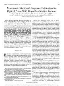
Fig. 3. The 100 best features selected by the KLT algorithm in the top image are shown as black squares in the top image. The bottom image shows how many features were tracked from the top image to the bottom image (corresponding to a robot translation of approximately 0.6 m.
The degree of match is the number of features successfully tracked from one image to the next. A total of 100 features are selected from each image and used for comparison. To take into account the possibility that two panoramic images might correspond to the same location but differ only in the orientation of the robot, the test image is rotated until the best match is found. Figure 3 shows the 100 best features identified in an image and shows how many of those features are successfully tracked to the lower image. This technique does not attempt to compute structure from motion on this data primarily because the additional complexity of tracking features for SFM would not be transferable to classes of sensors that do not return the necessary kind of information. While mapping, the mobile robot travels around an unknown area and stores images from its camera. The KLT algorithm and omnicamera setup is used as a “virtual sensor” that is used to compare images recorded at different locations along the trajectory of the robot. The output of this virtual sensor is a boolean value that determines whether or not the robot has returned to this location before. For the IEKF and batch ML algorithms compared in this paper, the accuracy of this
(15) 1 Originally
developed by Stan Birchfield at Stanford University [19].
measurement R = E{Nz NzT } is inferred by the locus of points (forming an ellipsoid) around a location, with the characteristic that the images recorded at each of them are considered identical by the KLT. When the received image does not match a previously recorded one, it is assumed that this location is novel and is added to the state vector of landmarks. This constitutes an exploration phase where the robot creates its world model. When the robot encounters an image which matches one that was previously seen, it considers these features to be the same and corrects its estimate of the landmark position. VI. O FFICE E NVIRONMENT E XPERIMENT The robot was moved around an environment in a path that intersected itself five times and an image was taken from the camera roughly every 0.3 m. The robot’s path is shown in Figure 4. (a) True path of the robot.
Fig. 4.
The path of the robot through the office environment.
The KLT algorithm was used to track features between each pair of images in order to find locations where the robot’s path crossed itself. Figure 5(a) shows the true path of the robot and the locations where the path crossed itself and landmarks were thus observed. Figure 5(b) shows the estimated path of the robot as computed by the robot’s noisy odometry readings. The estimated landmark positions observed during the run are shown as well. This figure does not assume that any sensor updates, i.e., location matchings, were made. A. Comparison of Estimators with Varying Noise Models A series of synthetic paths were generated from the above data set and used to test the performance of each of the estimators using different odometric noise models. The simulated odometric noise ranged from a standard deviation of 10 deg / sec to 120 deg / sec in encoder error (in 10 deg increments). A set of 100 robot paths were created for each noise variance setting. For each path, both of the robot’s wheel encoders were corrupted by noise drawn from a distribution with the same variance. Figure 6 shows the results of the different estimators on paths affected by increasing levels of odometric error. The batch ML estimator had the least amount of error in the placement of the landmarks, followed by the spring-based ML estimator. The performance of IEKF estimator was equivalent to the other estimators up to an error of around 50 deg / sec
(b) Estimated path of the robot.
Fig. 5. Real world experiments in an indoor environment (scale is in meters). Landmarks in the true path occur wherever there is an intersection in the path. Positions in the path are labeled chronologically.
but rapidly diminished in accuracy as the odometric errors increased. VII. C ONCLUSIONS & F UTURE W ORK The features and advantages of the various estimators are summarized in Table I. The complexity of the different estimators is computed as follows. The complexity of the IEKF is derived from the requirement of updating the covariance matrix, a matrix of M 2 entries, where M is the number of landmarks. The complexity of the batch ML algorithm is derived from the need to invert the covariance matrix. Finally, the spring-based ML algorithm ignores the cross-correlation
ACKNOWLEDGEMENTS Material based in part upon work supported by the National Science Foundation through grant #EIA-0224363, Microsoft Inc., and the Defense Advanced Research Projects Agency, MTO (Distributed Robotics), ARPA Order No. G155, Program Code No. 8H20, Issued by DARPA/under Contract #MDA97298-C-0008. R EFERENCES
Fig. 6. Comparison of the means and standard deviations of the three estimators on datasets with varying degrees of encoder error. Standard deviation of errors ranged from 10 deg / sec to 120 deg / sec.
terms and thus requires the inversion of only a diagonal matrix. This is much less time consuming than converting a full 2D covariance matrix.
Processing Complexity Advantages
Spring-Based ML Batch O(M ) Simple
Linearized Batch ML Batch O(M 3 ) Most accurate
IEKF Recursive O(M 2 ) Real-time
TABLE I C OMPARISON OF THE THREE ALGORITHMS .
As seen in the experimental section, the batch ML methods handles large amounts of system nonlinearity better than the recursive Kalman filter estimator. However, for relatively low levels of odometric error, the Kalman filter performed comparably to the batch estimators. The spring-based ML estimator did not perform as well because it did not reason explicitly about the errors in the distances between sensor readings of the same landmark (location). In terms of time complexity, the spring-based estimator was the simplest since it only had to iterate over the set of all readings. The primary advantage of the IEKF is that it is capable of handling all of the sensor readings as they are received. Although the method described in this paper uses images from an omnidirectional camera, main contributions of this approach (usage of the identity information by the filter) can be extended to any type of exteroceptive sensor that can be used for identifying an area (e.g. other sensors which measure the electro-magnetic, chemical, or audio signature of a location could also be used).
[1] P. E. Rybski, S. A. Stoeter, M. Gini, D. F. Hougen, and N. Papanikolopoulos, “Performance of a distributed robotic system using shared communications channels,” IEEE Transactions on Robotics and Automation, vol. 22, no. 5, pp. 713–727, Oct. 2002. [2] P. E. Rybski, F. Zacharias, J.-F. Lett, O. Masoud, M. Gini, and N. Papanikolopoulos, “Using visual features to build topological maps of indoor environments,” in Proceedings of the IEEE International Conference on Robotics and Automation, 2003, pp. 850–855. [3] P. E. Rybski, S. Roumeliotis, M. Gini, and N. Papanikolopoulos, “Appearance-based minimalistic metric SLAM,” in Proceedings of the IEEE/RSJ International Conference on Intelligent Robots and Systems, 2003, pp. 194–199. [4] T. Duckett, S. Marsland, and J. Shapiro, “Learning globally consistent maps by relaxation,” in Proceedings of the IEEE International Conference on Robotics and Automation, vol. 4, 2000, pp. 3841–3846. [5] A. Howard, M. Matari´c, and G. Sukhatme, “Localization for mobile robot teams using maximum likelihood estimation,” in Proceedings of the IEEE/RSJ International Conference on Intelligent Robots and Systems, EPFL Switzerland, Sept. 2002. [6] J. J. Leonard and H. F. Durrant-Whyte, “Mobile robot localization by tracking geometric beacons,” IEEE Transactions on Robotics and Automation, vol. 7, no. 3, pp. 376–382, 1991. [7] R. Smith, M. Self, and P. Cheeseman, “Estimating uncertain spatial relationships in robotics,” in Autonomous Robot Vehicles, I. J. Cox and G. T. Wilfong, Eds. Springer-Verlag, 1990, pp. 167–193. [8] S. Thrun, W. Burgard, and D. Fox, “A probabilistic approach to concurrent mapping and localization for mobile robots,” Machine Learning, vol. 31, pp. 29–53, 1998. [9] S. Thrun, D. Fox, W. Burgard, and F. Dellaert, “Robust monte carlo localization for mobile robots,” Artificial Intelligence, vol. 101, pp. 99– 141, 2000. [10] M. W. M. G. Dissanayake, P. Newman, S. Clark, H. F. DurrantWhyte, and M. Csorba, “A solution to the simultaneous localization and map building (SLAM) problem,” IEEE Transactions on Robotics and Automation, vol. 17, no. 3, pp. 229–241, June 2001. [11] J. Neira and J. Tards, “Data association in stochastic mapping using the joint compatibility test,” IEEE Transactions on Robotics and Automation, vol. 17, no. 6, pp. 890–897, Dec. 2001. [12] F. Dellaert and A. Stroupe, “Linear 2D localization and mapping for single and multiple robots,” in Proceedings of the IEEE International Conference on Robotics and Automation, May 2002. [13] R. Sim and G. Dudek, “Learning environmental features for pose estimation,” Image and Vision Computing, vol. 19, no. 11, pp. 733–739, 2001. [14] M. Betke and L. Gurvits, “Mobile robot localization using landmarks,” IEEE Transactions on Robotics and Automation, vol. 13, no. 2, pp. 251– 263, April 1997. [15] B. Kuipers and Y.-T. Byun, “A robot exploration and mapping strategy based on a semantic hierarchy of spatial representations,” Journal of Robotics and Autonomous Systems, vol. 8, pp. 47–63, 1991. [16] I. Ulrich and I. Nourbakhsh, “Appearance-based place recognition for topological localization,” in Proceedings of the IEEE International Conference on Robotics and Automation, San Francisco, CA, April 2000, pp. 1023–1029. [17] B. D. Lucas and T. Kanade, “An iterative image registration technique with an application to stereo vision,” Proceedings of the International Joint Conference on Artificial Intelligence, pp. 674–679, 1981. [18] C. Tomasi and T. Kanade, “Detection and tracking of point features,” School of Computer Science, Carnegie Mellon University, Tech. Rep., April 1991. [19] “KLT: An implementation of the Kanade-Lucas-Tomasi feature tracker.” http://robotics.stanford.edu/˜birch/klt/.