A Comparison of Microphone Phased Array Methods Applied to the Study of Airframe Noise in Wind Tunnel Testing Christopher J. Bahri and William M. Humphreys, Jr.ii NASA Langley Research Center, Hampton, Virginia 23681
Daniel Ernstiii , Thomas Ahlefeldtiv , and Carsten Spehrv German Aerospace Center DLR, D-37073 G¨ ottingen, Germany
Antonio Pereiravi , Quentin Lecl`erevii , and Christophe Picardviii University of Lyon - MicrodB, 69000 Lyon, France
Ric Porteousix The University of Adelaide, Adelaide, South Australia 5005, Australia
Danielle J. Moreaux, Jeoffrey Fischerxi , and Con J. Doolanxii The University of New South Wales, Sydney NSW 2052, Australia In this work, various microphone phased array data processing techniques are applied to two existing datasets from aeroacoustic wind tunnel tests. The first of these is from a large closed-wall facility, DLR’s Kryo-Kanal K¨ oln (DNW-KKK), and is a measurement of the high-lift noise of a semispan model. The second is from a small-scale open-jet facility, the NASA Langley Quiet Flow Facility (QFF), and is a measurement of a clean airfoil selfnoise. The data had been made publicly available in 2015, and were analyzed by several research groups using multiple analysis techniques. This procedure allows the assessment of the variability of individual methods across various organizational implementations, as well as the variability of results produced by different array analysis methods. This paper summarizes the results presented at panel sessions held at AIAA conferences in 2015 and 2016. Results show that with appropriate handling of background noise, all advanced methods can identify dominant acoustic sources for a broad range of frequencies. Lowerlevel sources may be masked or underpredicted. Integrated levels are more robust and in closer agreement between methods than narrowband maps for individual frequencies. Overall there is no obvious best method, though multiple methods may be used to bound expected behavior. i Research
Engineer, Aeroacoustics Branch, Senior Member AIAA,
[email protected] Engineer, Adv. Measurements and Data Systems Branch, Associate Fellow AIAA,
[email protected] iii Research Engineer, Institute of Aerodynamics and Flow Technology - Experimental Methods,
[email protected] iv Research Engineer, Institute of Aerodynamics and Flow Technology - Experimental Methods,
[email protected] v Research Engineer, Institute of Aerodynamics and Flow Technology - Experimental Methods,
[email protected] vi Postdoctoral Researcher, Laboratoire de M´ ecanique des Fluides et d’Acoustique, EC Lyon,
[email protected] vii Assistant Professor, Laboratoire Vibrations Acoustique, INSA Lyon,
[email protected] viii Research Engineer, MicrodB,
[email protected] ix Ph.D. Candidate, School of Mechanical Engineering,
[email protected] x Lecturer, School of Mechanical and Manufacturing Engineering, Member AIAA,
[email protected] xi Research Associate, School of Mechanical and Manufacturing Engineering, Member AIAA,
[email protected] xii Associate Professor, School of Mechanical and Manufacturing Engineering, Senior Member AIAA,
[email protected] ii Research
1 of 18 American Institute of Aeronautics and Astronautics
Nomenclature CLEAN CLEAN-SC DAMAS DR M N NNLS SADA α Γ ν
Radio astronomy deconvolution algorithm CLEAN based on spatial Source Coherence Deconvolution Approach for the Mapping of Acoustic Sources diagonal removal Mach number grid point count Nonnegative Least Squares Small Aperture Directional Array Angle of Attack (deg) Dihedral angle (deg) functional beamforming exponent
I.
Introduction
ecently, the microphone phased array community has come together in an attempt to document and R better understand the accuracy and variability of many data processing techniques. Many members of the field recognize that, with the wide variety of beamforming and deconvolution techniques available, common datasets are necessary for both qualitative and quantitative analysis of these methods. Common datasets can be used to compare the various existing techniques, evaluate the variability of each technique to its implementation and input parameters, and provide a mechanism for testing new techniques. The community held a kick-off meeting at the 20th American Institute of Aeronautics and Astronautics/Council of European Aerospace Societies (AIAA/CEAS) Aeroacoustics Conference in Atlanta, Georgia in June of 2014. At the meeting, participants discussed the characteristics required of a benchmark dataset, as well as the various types of data that could be considered. Within the interest range of experimental aeroacoustics, sources may be discrete or distributed, may have arbitrary levels of distributed coherence, and may experience unknown reflection, refraction, and reverberance. Ideally, benchmark datasets would isolate and address each of these conditions. Three types of benchmark dataset cases were discussed: analytic, computational, and experimental. Analytic benchmarking cases contribute value through having known solutions against which each analysis method could be compared. Computational cases contribute value by being closer to experiments in complexity while retaining at least a well-approximated reference solution. Cases stemming from a well-documented and controlled experiment provide a common baseline of real data for comparison of methods and establish overall bounds and variability of the array methods considered. Since the initial meeting, a suite of cases has been released to the community for study. Panel sessions have occurred at the 21st and 22nd AIAA/CEAS Aeroacoustics Conferences, where interim results for these cases were presented and discussed. Several of the original cases have now received sufficient attention to warrant publication of the results. Two of the experimental cases, labeled ‘DLR 1’ and ‘NASA 2’, are addressed in this work. Both of these cases are datasets from airframe noise wind tunnel tests, though with different problem scales. A companion paper considers two of the analytic datasets.1
II.
Case: DLR 1
The DLR benchmark problem consists of a test configuration with a Dornier-728 semispan (or half) model in high-lift configuration in the cryogenic wind tunnel at the DLR Cologne site (Kryo-Kanal Koeln, DNW-KKK). The details of this test have been documented previously.2 II.A. II.A.1.
Case description General setup
The DNW-KKK is a continuous flow low-speed wind tunnel with a 2.4 m × 2.4 m closed wall test section. By injection of liquid nitrogen, the wind tunnel can be operated in the range of 100 K < T < 300 K at Mach numbers up to 0.38. It should be noted that the wind tunnel was operated at ambient conditions in this benchmark case.
2 of 18 American Institute of Aeronautics and Astronautics
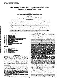
The microphone array contains 144 microphones, each one recessed behind a cone and arranged in spiral arms with an array aperture of 1 m × 1 m. The dimensions of the array fairing are 1756 mm in the streamwise and 1300 mm in the vertical (normal to the flow) direction. The array protrudes 25 mm into the test section. The leading and the trailing edges have a slope of 6◦ to reduce disturbances due to flow separation. Fig. 1 shows the test setup. The array is mounted onto the sidewall, and the Dornier-728 semispan model is located in the center of the test section. The model of scale 1:9.24 is arranged in a landing configuration and has a mean aerodynamic chord length of 0.353 m and a semispan width of 1.44 m. Boundary layer trips are only applied to the nacelle and not the rest of the model. On the leading edge, the slat angle is 26.3◦ , and the Krueger flap angle is 80◦ . On the trailing edge, the flap angle is 35◦ , and the aileron has an angle of 0◦ . The microphone signals are simultaneously sampled with an A/D conversion of 16 bits at a sampling frequency of 120 kHz by a data acquisition system located outside the test section. The recording time for each measurement is 30 s. To reduce influence of the low frequency wind tunnel noise, a second-order high-pass filter with a cut-off frequency of 500 Hz was used (compensated for in the processing afterward). For the benchmark case, the model’s angle of attack is α = 3◦ and the free stream velocity is 87.97 m/s (M = 0.25). Table 1 summarizes the general measurement conditions.
Figure 1. Photo of the test section with the array mounted on the side wall and the DO-728 semispan model in the center, view in the flow direction.
Table 1. DLR1 measurement conditions. Configuration High-Lift
II.A.2.
Free Stream Velocity 87.97 m/s
Angle of Attack 3◦
Recording Time 30 s
Geometric details
The source maps are calculated on an equidistant discrete grid shown in Fig. 2. The grid covers the region of interest in an observation plane of 1.05 m × 1.45 m of the semispan model. In order to reduce the computational effort for the more costly algorithms, the grid resolution was set to dxz = 20 mm. This led to 3869 scanning points for the baseline grid, though some contributors altered the grid layout slightly. The initial grid is in the (x,z)-plane and has a distance of ∆y = 1.045 m (position of the wing root) to the microphone array. The microphone array is in the (x,z)-plane with the center microphone position at (x,y,z) = (0 m, 0 m, 0 m). For the calculation, the initial scanning grid is rotated by:
3 of 18 American Institute of Aeronautics and Astronautics
1. the mean dihedral angle of the wing Γ = 6.5◦ , rotation axis x, point of rotation (x,y,z) = (0 m, 1.045 m, -0.675 m) 2. the angle of attack α = 3◦ , rotation axis z, point of rotation (x,y,z) = (0.130 m, 1.175 m, -0.902 m).
Figure 2. Scanning grid of the source map calculations and the microphone positions in the (x,z)-plane. The location of the semispan model is sketched in the background.
II.A.3.
Model details and acoustic sources
A photo and a sketch of the windward side of the semispan model is given in Fig. 3. On the leading edge, the slats (not slotted) with seven tracks and the Krueger flap with two tracks can be seen. Here noise sources can be expected to originate from the tracks, the slat horn (inboard slat side edge) and the gap between the Krueger flap and the fuselage. At the low Reynolds numbers, also, tonal noise originating from different slat cove noise mechanisms may occur.2 On the trailing edge, the flaps (not slotted) with three tracks and an extension of the nacelle mount can be seen. Here noise sources can be expected at the flap side edge and the flap tracks. Additional noise originating from the wing tip or nozzle flow in the flap gap occurs less often. Furthermore, there can be sources from strakes (on the nacelle), interactions of the nacelle mount with the accelerated nozzle flow, and other parasitic noise sources (i.e., cavities). From the results in previous work,2 it is known that the flap side edge becomes a relevant source in the frequency range of 6 to 15 kHz. Therefore, the frequency 8496 Hz is chosen for comparing source maps, and an integration area around the flap side edge is indicated by the blue rectangle in Fig. 3.
4 of 18 American Institute of Aeronautics and Astronautics
Figure 3. A detailed view of the lower surface of the wing as installed in the tunnel (left) and sketch (right). The integration area for the flap side edge is indicated by the blue rectangle.
II.B.
Algorithms
A brief summary of the different algorithms that were applied to the benchmark case DLR 1 is given here. The first, the conventional beamformer, is the standard algorithm, and the result is usually called the dirty map. It is calculated by weighting and summation over all cross correlation coefficients.3 Functional Beamforming was proposed by Dougherty4 and is a generalization of the conventional and minimum variance beamformer (or Capon beamformer). A matrix function is applied to the cross spectral matrix, and the beamforming output is normalized by the inverse of this function. For functional beamforming, the matrix function is f (x) = xν . In theory, this algorithm decreases all sidelobes by an arbitrary factor without any significant additional computational effort. CLEAN-SC is a maxima-seeking algorithm to deconvolve the dirty map into incoherent source points and was developed by Sijtsma.5 The computational effort is about twice that for conventional beamforming. DAMAS is a deconvolution algorithm that tries to solve a Nonnegative Least Squares (NNLS) system with a modified Gauss-Seidel method and was developed for aeroacoustics by Brooks and Humphreys.6 In general, the NNLS system can be solved with several suitable techniques, for example those given by Bro and de Jong7 or by Lawson and Hanson.8 Since NNLS and DAMAS are working on dense matrices of size N × N , where N is the number of scanning points, the computational effort increases quadratically with N . The last algorithm is a Bayesian approach to the inverse method problem, which combines physical and probabilistic assumptions about the source field, developed by Pereira et al.9 II.C. II.C.1.
Results Comparison of source maps at one narrowband frequency
In Figs. 4a and 4b, the source maps of conventional beamforming and functional beamforming with exponent ν = 30 are shown. The peak level in the functional source map is reduced by about 2 dB, and the map is nearly sidelobe-free. This suggests that every part of the functional map corresponds directly to an expected
5 of 18 American Institute of Aeronautics and Astronautics
source. The CLEAN-SC source map contributed by DLR (Fig. 4c) contains exactly one source on every slat track and one source on the flap side edge. This result is quite similar to the algorithms NNLS and Bayes from the University of Lyon, but the CLEAN-SC source map is slightly more sparse than their NNLS and Bayes results (see Fig. 4d). Next, the DAMAS results from NASA and DLR are compared in Figs. 5a and 5b. The peak level differs by 1 dB. While the same algorithm is used on the same measurement data, there are differences in the result. Overall the deconvolution images look similar. Possible reasons for the differences could be the slightly different scanning grid and a different sweep strategy in the Gauss-Seidel iteration. Compared to the functional source map, the DAMAS source maps appear much noisier. A typical artifact for DAMAS is that sources are placed on the edge of the scanning grid because there are sources in the measurement outside the scanning grid. NASA contributed a version of DAMAS where the diagonal is removed by an eigenvector-based subtraction technique,10 but at the selected frequency there is little difference compared to ordinary diagonal removal (see Fig. 5c). The NNLS algorithm contributed by DLR (Fig. 5d) shows slightly fewer sources, but has nearly the same peak level as DAMAS from DLR. However, the NNLS solution by the University of Lyon (Fig. 5e), looks like a clean source map with sources only on the slat track and one on the flap side edge. On the slat just outboard of the engine mount, the sources are densely distributed. The peak level is 3 dB higher than the same algorithm from DLR. The huge difference between these source maps can be explained by the different definitions of the point spread function that are used in the deconvolution process. In the DLR solution, diagonal removal was applied, respectively, on the dirty map as well as on the point spread function, whereas the NNLS solution by the University of Lyon uses a point spread function without diagonal removal (though it is still applied to the dirty map). In Figs. 5f and 5g, DAMAS and NNLS are applied by DLR with the constraint that the point spread function has to be nonnegative. With this constraint, both algorithms give back much sparser source maps. One further modification is that no diagonal removal is applied on the point spread function. This means that a dirty map with diagonal removal is deconvolved with a point spread function without diagonal removal. This leads to similar source maps like the NNLS results from the University of Lyon (compare Figs. 5h and 5i with 5e). It can be concluded that the source maps differ because of the different definitions of the point spread function. This is to be expected, as altering the linear system of equations solved by DAMAS and NNLS should change each algorithm’s output. II.C.2.
Comparison of integrated spectra of the flap side edge
The integrated spectra for the isolated flap side edge (see Fig. 6) are now compared. Since this is a measurement of a realistic model, the true source power is not known. For all deconvolution type algorithms, the source map is summed up across the area indicated in Fig. 3. The source maps of the conventional and functional beamformer are summed up as well and normalized with a point spread function in the center of the integration area.11 When comparing the integrated spectra in all plots in Figs. 6a - 6d, it is clear that in the frequency range between 7 and 13 kHz, where the source level of the flap side edge is dominant, all algorithms have nearly the same level. The difference here is only 2-3 dB between all algorithms, with the exception of functional beamforming in Fig. 6a. Below 10 kHz, the functional beamforming integrated values are up to 10 dB higher than all other algorithms. The cause for this is still under investigation. At around 5 kHz, advantages to NNLS and DAMAS over CLEAN-SC are evident (see Figs. 6b and 6c), although even these methods show variability. The resolution of CLEAN-SC is limited to the peak values of the conventional beamformer, and there are only isolated frequencies where CLEAN-SC finds a source in the integration area. However, the conventional beamforming integrated values are similar to the values of NNLS and DAMAS (see Figs. 6c and 6d). Here it is evident that integrated values at low frequencies from conventional beamforming are more robust than those from CLEAN-SC. At frequencies below 3 kHz, the results from the conventional and functional beamforming are more than 20 dB higher than the deconvolution results, where no source is found in the flap side edge integration area (see Figs. 6a and 6d). While true source power in this frequency range is unknown, it may be bounded with knowledge of the behavior of the various algorithms. The integrated levels of the conventional and functional algorithms are highly affected by the background noise of the wind tunnel, so the true level of the results is expected to have values between these and the deconvolution methods. In the frequency range of 15 to 40 kHz, the DAMAS and NNLS algorithms coincide with the conventional integrated values (within 3-4 dB), but only if the point spread function and dirty map are allowed to be 6 of 18 American Institute of Aeronautics and Astronautics
Contributor: DLR Algorithm: Conventional - DR Peak: 52.84 dB
Contributor: DLR Algorithm: FUNCTIONAL(30) - DR Peak: 50.74 dB 52
50
0.6
48
50
46 44
0
42
-0.2
40 38
-0.4
46 44
0.2
42
0 40
-0.2
38
-0.4
36 34
36
-0.6
-0.6 32
34
-0.2
0
0.2 x [m]
0.4
0.6
-0.2
0
(a)
0.2 x [m]
0.4
0.6
(b)
Contributor: DLR Algorithm: CLEAN-SC - DR Peak: 52.79 dB
Contributor: Univ. of Lyon Algorithm: Bayes - DR - L0.9 Peak: 50.38 dB 50
52
0.6
0.6 48
46
z [m]
0.2
44
0 42
-0.2
40
-0.4
38
0.4
46
0.2
44 42
z [m]
48
PSD [dB] rel. 2 10 -5 Pa
50
0.4
0
40
-0.2
38 36
-0.4
34
36
-0.6
-0.6
32
34
-0.2
0
0.2 x [m]
0.4
PSD [dB] rel. 2 " 10-5 Pa
z [m]
0.2
z [m]
48
0.4
PSD [dB] rel. 2 " 10-5 Pa
0.4
PSD [dB] rel. 2 " 10-5 Pa
0.6
0.6
-0.2
0
(c)
0.2 x [m]
0.4
0.6
(d)
Figure 4. Power spectral density source maps of the Do728 semispan model at the narrowband frequency 8496 Hz with a dynamic range of 20 dB.
7 of 18 American Institute of Aeronautics and Astronautics
Contributor: NASA Algorithm: DAMAS - DR Peak: 50.38 dB
Contributor: DLR Algorithm: DAMAS - DR Peak: 49.34 dB
Contributor: NASA Algorithm: DAMAS - Eigenvector Based DR Peak: 50.47 dB
50
0.6
0.6
50
0.6
48
48
-0.2
38 36
-0.4
40
0
38
-0.2 36
-0.4
0.4
46
0.2
44 42
0 40
-0.2
38 36
-0.4
34
34
-0.6
PSD [dB] rel. 2 " 10-5 Pa
40
z [m]
0
42
PSD [dB] rel. 2 " 10-5 Pa
z [m]
42
44
0.2
z [m]
44
Pa
0.2
48 46
0.4 -5
46
PSD [dB] rel. 2 " 10
0.4
34 32
-0.6
32
-0.6
32
30
0.2 x [m]
0.4
0.6
-0.2
0
(a)
0.2 x [m]
0.4
0.6
-0.2
0
(b)
Contributor: DLR Algorithm: NNLS - DR Peak: 49.11 dB 48
0.4
0.6
(c)
Contributor: Univ. of Lyon Algorithm: NNLS - DR Peak: 51.99 dB
0.6
0.2 x [m]
0.6
Contributor: DLR Algorithm: DAMAS - DR PSF>0 Peak: 49.78 dB 0.6
50
48
46
0.4
-0.2
36
-0.4
34
0.2
44
0
42
-0.2
40 38
-0.4
46 44
0.2 42
z [m]
38
46
PSD [dB] rel. 2 " 10-5 Pa
40
0
-5
42
z [m]
z [m]
0.2
PSD [dB] rel. 2 " 10
44
0.4
48
Pa
0.4
0
40 38
-0.2
36
-0.4
34
36 32
-0.6
-0.6
32
-0.6
34
30
30
32
-0.2
0
0.2 x [m]
0.4
0.6
-0.2
0
(d)
0.2 x [m]
0.4
0.6
-0.2
0
(e)
Contributor: DLR Algorithm: NNLS - DR PSF>0 Peak: 49.86 dB
0.2 x [m]
0.4
0.6
(f)
Contributor: DLR Algorithm: DAMAS - DR PSF>0 NoPsfDR Peak: 50.05 dB
Contributor: DLR Algorithm: NNLS - DR PSF>0 NoPsfDR Peak: 50.58 dB
50
42
0
40 38
-0.2
36
-0.4
34 32
-0.6
48
0.4
Pa
46 44
0.2
42
z [m]
0.2
PSD [dB] rel. 2 " 10
-5
44
0.4
0
40 38
-0.2
36
-0.4
50
0.6
48
46 44
0.2
z [m]
46
0.4
z [m]
0.6
48
PSD [dB] rel. 2 " 10-5 Pa
0.6
PSD [dB] rel. 2 " 10-5 Pa
0
42
0 40
-0.2
38 36
-0.4
34
-0.6
32
PSD [dB] rel. 2 " 10-5 Pa
-0.2
34
-0.6
32
30
-0.2
0
0.2 x [m]
(g)
0.4
0.6
-0.2
0
0.2 x [m]
0.4
0.6
(h)
-0.2
0
0.2 x [m]
0.4
0.6
(i)
Figure 5. Power spectral density source maps of the Do728 semispan model at the narrowband frequency 8496 Hz with a dynamic range of 20 dB for all DAMAS and NNLS algorithms. PSF>0 means that the point spread function was forced to be nonnegative. NoPsfDR means that no diagonal removal was applied on the point spread function.
8 of 18 American Institute of Aeronautics and Astronautics
negative (see Figs. 6c and 6d). If the point spread function and dirty map are treated to be nonnegative, the NNLS algorithm results in much lower integrated levels that coincide with the Bayesian algorithm from University of Lyon and CLEAN-SC from DLR (compare Figs. 6b and 6d). The constraint that the point spread function should be nonnegative causes the deconvolution A-matrix to have a higher rank, which could be seen as some kind of regularization. Again, the exact source power is not known, but it is currently assumed that integrated values of CLEAN-SC, NNLS with nonnegativity constraint and the Bayes algorithm yield more appropriate results at the frequency range above 15 kHz. As a final note, it is observed that the NASA and DLR implementations of DAMAS yield nearly identical spectra for the entire bandwidth of interest. While this does nothing to validate the levels output by DAMAS, it does help validate the consistency of DAMAS as minor implementation details have minimal effect on the computed integrated spectra. II.D.
Case Discussion
All algorithms described above are discussed with respect to their limitations and applicability to this benchmark case. This is done with regard to two criteria: 1. Is it possible to extract the position of all expected aeroacoustic sources from the beamforming map at 8496 Hz, where the flap side edge is a significant noise source? Sources are expected to occur at every slat track and the flap side edge. The source strength is unknown. 2. What is the dynamic range of the beamforming map at 8496 Hz? The dynamic range is defined here as the maximum in the source map minus the loudest source position that is not found on the semispan model, for example spurious sources related to the wind tunnel background noise. The following statements are only valid for the narrowband frequency of 8496 Hz and the chosen grid resolution of dxy = 20 mm, and with diagonal removal applied to manage background noise contamination. • Conventional Beamforming: All sources are visible. In some cases however, several sources that are believed to occur individually (individual slat tracks) fuse together to form a single large source due to the spatial limitation of the point spread function. The dynamic range of the beamforming map is approximately 10 dB. • Functional Beamforming: Functional beamforming is the only algorithm that identifies sources on the flap tracks, but it is not known if these are real source positions. It is not possible to discriminate between all source positions. The dynamic range is approximately 20 dB. • CLEAN-SC: All sources are identified separately and the dynamic range exceeds 20 dB. • Bayes: All sources are identified separately and the dynamic range exceeds 20 dB. • DAMAS: For this algorithm, diagonal removal has to be applied to the point spread function in addition to the beamformer output. All sources are identified but the dynamic range only reaches 10 dB. • NNLS: Applied without diagonal removal on the point spread function, this algorithm is capable of separating all sources and providing a dynamic range of approximately 20 dB. Due to the unknown strength of the source at the flap side edge, it is not possible to assess the quality of the different integrated spectra with regard to a correct answer. As described above, in the frequency range between 7 kHz and 15 kHz where the source level of the flap side edge is dominant, all algorithms produce a similar output level. Consequently, if an aeroacoustic source on a complex model is dominant, the source strength is reconstructed within a variation of 3 dB between all algorithms, except for functional beamforming. The variation of 3 dB between all the algorithms leads to one consequence in the process of wind tunnel data analysis: if only small modifications are made to the model, the analysis should be 9 of 18 American Institute of Aeronautics and Astronautics
65
65 DLR, Conventional - DR DLR, CLEAN-SC - DR DLR, FUNCTIONAL(30) - DR
60
55
55
50
50
PSD [dB] rel. 2 10 -5 Pa
-5 PSD [dB] rel. 2 10 Pa
60
DLR, Conventional - DR DLR, CLEAN-SC - DR Univ. of Lyon, Bayes - DR - L0.9
45
40
35
45
40
35
30
30
25
25
20
20 5
10
15 20 25 Frequency [kHz]
30
35
40
5
10
15 20 25 Frequency [kHz]
(a)
35
40
(b)
65
65 DLR, Conventional - DR DLR, DAMAS - DR NASA, DAMAS - DR NASA, DAMAS - Eigenvector Based DR DLR, DAMAS - DR PSF>0 DLR, DAMAS - DR PSF>0 NoPsfDR
60
DLR, Conventional - DR DLR, NNLS - DR Univ. of Lyon, NNLS - DR DLR, NNLS - DR PSF>0 DLR, NNLS - DR PSF>0 NoPsfDR
60 55
PSD [dB] rel. 2 " 10 -5 Pa
55
PSD [dB] rel. 2 " 10 -5 Pa
30
50 45 40 35
50 45 40 35
30
30
25
25
20
20 5
10
15 20 25 Frequency [kHz]
30
35
40
5
10
15 20 25 Frequency [kHz]
(c)
(d)
Figure 6. Integrated spectra over the flap side edge area (see Fig. 3).
10 of 18 American Institute of Aeronautics and Astronautics
30
35
40
performed solely by comparing the results of only one algorithm. For dominant airframe noise sources such as the flap side edge between 7 kHz and 15 kHz, various algorithms all are in close agreement. However, comparison and quantification of levels resulting from sources that are not dominant remains difficult, as seen in the variability of the integrated levels above 15 kHz (see figure 6). For airframe noise, the problem can be modeled very well with the incoherent monopole assumption. For the model used in the current evaluation, most of the aeroacoustic sources have small source regions, and a sparse solution is expected. As such, the CLEAN-SC and Bayes algorithms work well on an airframe model, since they assume a sparse source distribution. Such a result may not hold as well for more distributed sources, as seen in the NASA 2 case.
III.
Case: NASA 2
The NASA 2 case is a dataset from a small-scale open-jet wind tunnel experiment, where a clean (no highlift devices deployed) airfoil at α = −1.2◦ , the angle of attack at which it generates zero lift, was immersed in a Mach 0.17 flow. As the airfoil was installed in a clean configuration, noise sources are expected from the model trailing edge and the leading edge trip region. This dataset was selected for the effort as it has a wide dynamic range of the model and background acoustic sources of interest, has a well-behaved background noise measurement, allows for analysis of free shear layer propagation models, and has minimal self-noise microphone contamination. III.A.
Case description
This benchmark case, described in detail in previous studies of trailing edge noise measurements12 as well as in the original DAMAS work,6 consists of a test configuration where an NACA 63-215 Mod-B full-span airfoil, with a 16-inch (0.406 m) chord length and 36-inch (0.914 m) span was mounted at its zero-lift angle of attack of α = −1.2◦ relative to the vertical flow in the NASA Langley Quiet Flow Facility (QFF). A photograph of the installation is shown in Fig. 7a, and a schematic of the particular acquisition of interest in Fig. 7b. The photograph shows the airfoil mounted vertically in the test section with sidewalls partially removed for visibility (shown here with a half-span flap, which was removed for the benchmark case of interest). The rotating boom, on which the 33-microphone Small Aperture Directional Array (SADA)13 is mounted, is positioned in the bottom-right of the photograph. For both the photograph and the schematic, flow is from the bottom to the top of the image. The model had a spanwise uniform sharp trailing edge of 0.005-inch (0.127 mm) thickness. Grit of size #90 was distributed along the leading edge over the first 5% of the model to ensure a fully turbulent boundary layer at the trailing edge. The SADA was positioned at an elevation angle of 90◦ with respect to the pressure side of the model, referenced to the test section downstream direction. Data were acquired with the SADA at a test section Mach number of M = 0.17. Data were acquired at a sampling period of 7 µs, corresponding to a sampling rate of just under 143 kHz. A total of 2,048,000 samples were acquired simultaneously for each microphone channel. Table 2 summarizes the general measurement conditions. Table 2. NASA2 measurement conditions. Configuration Clean
Free Stream Mach 0.17
Angle of Attack -1.2◦
Recording Time 14.3 s
Given the zero-lift condition of the model, it was assumed that the mean shear layer bounding the test section flow remained attached to the nozzle lip line, was planar, and was located a constant distance (12 inches or 0.305 m) from the centerline of the test section on either side of the model. The model itself was offset from the tunnel centerline by 5.25 inches (0.133 m), and the SADA was located 60 inches (1.524 m) from the model trailing edge. Corresponding background data were acquired using the SADA at the same position with the model removed from the facility (still retaining the test section side plates). III.B.
Metrics and contributions
Processed data from microphone phased arrays can be compared both qualitatively and quantitatively. For both qualitative and quantitative evaluation, submitted results are compared with the original published
11 of 18 American Institute of Aeronautics and Astronautics
(a) Installation photograph14
(b) Experiment schematic
Figure 7. Installation and measurement layout of the NACA 63-215 Mod-B trailing edge noise measurement in QFF.
DAMAS results.6 The original results are not treated as “correct,” but do provide an anchor for evaluation. Qualitatively, contributions are evaluated in terms of source isolation on a one-third octave band basis. The separation and focusing of the leading and trailing edge noise sources can be considered as a function of frequency. Quantitatively, the integrated power (per-foot-span) of the leading and trailing edge sources can be computed at the center of the SADA and compared to the existing results. Note that a suggested beamforming grid is provided with the case, but not required for contributions. Three organizations contributed processed results for the NASA 2 case. The first, NASA Langley Research Center, revisited DAMAS using various combinations of diagonal removal and background subtraction techniques.10 The Langley contributions used the supplied microphone shading scheme.13 The second, University of Lyon, applied DAMAS, deconvolution using an NNLS solver, and an inverse method using Sparse Bayesian Reconstruction.9 The Lyon contributions applied no microphone shading and applied the same eigenvalue background subtraction technique as some of the Langley contributions. The third, University of New South Wales (UNSW), contributed analysis using both conventional beamforming and CLEAN-SC.5 The UNSW contributions applied no microphone shading and applied a conventional subtraction technique to deal with the facility background noise. All of the contributions corrected for the open-jet shear layer effects using Amiet’s method.15 The variety of included diagonal removal, background subtraction, and microphone shading combinations preclude the isolation of individual effects on the selected algorithms, but do allow the assessment of variability across what might be considered “best practices” for each contributor. III.C. III.C.1.
Results Qualitative analysis - source map comparison
The 12.5 kHz one-third octave bands of the submissions are considered. From the original DAMAS work, this frequency band shows significant energy from both the leading and trailing edge sources. They are separated from each other by more than the 3-dB beamwidth of the array, but not by a significant margin. A subset of these 12.5 kHz source maps is shown in Fig. 8. While more contributions were received than are plotted here, this selection highlights the major features and behaviors of the submissions. For all of these plots, flow is from the bottom of the figure to the top (in the positive-x direction). The vertical black lines at y = ±0.46 m indicate the test section sidewalls. The horizontal black lines at x = 0.6 m and 1 m indicate the respective leading and trailing edges of the airfoil model. The NASA Langley contributions are shown in Fig. 8a and Fig. 8b. All three of the NASA contributions appear largely similar, with minor variations in the low-level spurious sources. The selected subset compares the two subtraction methods in ways they are likely to be used. Conventional subtraction, when applying
12 of 18 American Institute of Aeronautics and Astronautics
diagonal removal, (Fig. 8a) protects from negative autospectral terms contaminating the initial conventional beamforming step of DAMAS. Eigenvalue subtraction, when including the cross spectral matrix diagonal, (Fig. 8b) leverages the method’s ability to preserve the positive semidefinite nature of the cross spectral matrix and thus the positive semidefinite nature of the point spread function. Both methods not only successfully separate the leading and trailing edge sources visually, but match peak levels to the second decimal place. Note that the selected DAMAS grid sweep strategy tends to push the acoustic energy of reflections from the hard test section sidewalls toward the y-boundaries of the grid. This has been observed independently in other applications of DAMAS.16 The University of Lyon contributions are shown in Fig. 8c and Fig. 8d. While Lyon submitted five advanced methods in addition to one-third octave images for conventional beamforming, the selected two illustrate the character of the various submissions. The Bayesian method shown in Fig. 8c successfully identifies the leading and trailing edge sources and shows almost no low-level spurious sources, although it concentrates energy near the model center span and test section sidewalls. Note that the nature of the Bayesian method makes it difficult to directly relate the peak level of this technique to the other images. Additional scaling is applied in the spectral reconstruction process for subsequent quantitative comparison. The DAMAS results shown in Fig. 8d also separate the leading and trailing edge sources. These results have fewer low-level spurious sources than the equivalent NASA analysis, but also show leading and trailing edge source distributions that are likely too sparse for the expected characteristics. This difference could be due to iteration count, sweep direction, or details of the calculation of the propagation and steering vectors. The UNSW contributions are shown in Fig. 8e and Fig. 8f. As expected, since the leading and trailing edge of the airfoil are separated by more than the SADA’s 3-dB beamwidth at this frequency, conventional beamforming can successfully separate the leading and trailing edge noise sources. However, the dynamic range of Fig. 8e must be reduced to 6 dB to visually isolate the sources. Additionally, due to the distributed characteristics of the sources, the peak level of the map is dramatically higher than any of the other analysis techniques. The CLEAN-SC results shown in Fig. 8f successfully separate the leading and trailing edge noise sources on a 20-dB scale, with almost no low-level spurious sources. However, like the Bayesian L1 method, it tends to concentrate energy near the model center span and test section sidewalls. III.C.2.
Quantitative analysis - integrated source spectra
Integrated spectra for the leading edge trip tape are shown in Fig. 9 and for the trailing edge in Fig. 10. The metrics considered are the leading and trailing edge source powers, per foot span, at the center of the SADA array. Individual contributors were allowed to choose their own process for computing these metrics from their algorithm results. These results are compared to the originally-published DAMAS results, which retain their labels from the initial publication: ‘DAMAS STD’ for no diagonal removal, and ‘DAMAS DR’ for diagonal removal. The leading edge spectra in Fig. 9 all show similar shape between 10 kHz and 40 kHz, lending some confidence to the qualitative spectral shape and level computations. The maximum spread in results for this frequency band is just below 6 dB at 40 kHz. The close level calculations at 12.5 kHz show that many of the differences in the qualitative maps tend to average out for a source integration procedure. Below 10 kHz, all of the advanced algorithms trend similarly but integrated conventional beamforming can no longer separate the sources and diverges from the rest of the predictions. This is evident as the spectral level and shape for the conventional beamforming integrated leading edge spectrum follow the spectral level and shape for the conventional beamforming integrated trailing edge spectrum in Fig. 10. Below approximately 7 kHz, the advanced techniques start showing divergence in both spectral level and shape. The divergence becomes particularly significant by 5 kHz, spanning well over 10 dB, with differing level trends. This indicates a limitation in what can be expected from many of these advanced analysis techniques. The SADA array was designed to have a 1 foot main lobe at 10 kHz,13 so at frequencies less than half of that, even advanced methods may have difficulty, or at least show significant disagreement, in how multiple source contributions are separated. The difficulty may be exacerbated by the fact that most estimates of the trailing edge noise source are more than 10 dB above the estimates of the leading edge noise source in this frequency range. The companion simulated analysis shows that significant variability may be present in array results when a strong source is present near a weak source.1 At frequencies above 40 kHz, levels diverge. Spectral trends, however, split into two groups, separated by the application of diagonal removal. This behavior of diagonal removal, for which computed levels are above what would be expected based on other data from the facility, has sometimes been observed experimentally 13 of 18 American Institute of Aeronautics and Astronautics
Contributor: NASA Algorithm: DAMAS - DR, Conv. Sub; Peak: 31.53 dB 1.6
Contributor: NASA Algorithm: DAMAS - No DR, Eig. Sub; Peak: 31.53 dB 1.6
30
20
0.8 0.6
1 20
0.8 0.6
15
0.4
15
0.4 0
0.5
-0.5
y [m]
0
(a)
(b)
Contributor: Univ. of Lyon Algorithm: Bayes - DR - L1 Eig. Sub; Peak: 18.69 dB
Contributor: Univ. of Lyon Algorithm: DAMAS - No DR Eig. Sub; Peak: 36.38 dB
1.6
1.6 15
10
1 0.8
5
30
1.2
x [m]
1.2
35
1.4 dB rel 2 10-5 Pa
1.4
1 25
0.8
0.6
0.6 0
0.4 -0.5
0
20
0.4
0.5
-0.5
y [m]
0
0.5
y [m] (c)
(d)
Contributor: UNSW Algorithm: Conventional - DR Conv. Sub; Peak: 44.84 dB
Contributor: UNSW Algorithm: CLEAN-SC - DR Conv. Sub; Peak: 38.94 dB
1.6
1.6 44
1.2
1.4
1
42
0.8
41
0.6
40
0.6
0.4
39
0.4
-0.5
0
35
1.2
x [m]
43
dB rel 2 10-5 Pa
1.4
30
1 0.8
0.5
25
20
-0.5
y [m]
dB rel 2 10-5 Pa
x [m]
0.5
y [m]
dB rel 2 10-5 Pa
-0.5
x [m]
dB rel 2 10-5 Pa
1
25
1.2
x [m]
25
1.2
x [m]
30
1.4 dB rel 2 10-5 Pa
1.4
0
0.5
y [m] (e)
(f)
Figure 8. Qualitative comparison of a subset of the NASA 2 contributions. Results shown are for the 12.5 kHz one-third octave band. All maps aside from conventional beamforming are set to a 20-dB scale.
14 of 18 American Institute of Aeronautics and Astronautics
at high frequencies when applying DAMAS, but the exact cause has not been determined. The behavior does appear with both the Lyon DAMAS and NNLS contributions, though the Bayesian method appears unaffected. Note that the disagreement between the NASA data with diagonal removal from 2004 and the updated submission, which is minor between 6 kHz and 40 kHz, is attributed to differences in grid density, grid traversing pattern, and iteration count in the processing of these two cases. The trailing edge spectra in Fig. 10 show more uniform qualitative agreement than the leading edge spectra for 2 kHz and beyond, likely due to the dominance of the trailing edge noise over the leading edge noise at these low frequencies. The one exception to this behavior is an outlying low-power estimate for the NASA-provided eigenvalue subtraction method at 1.25 kHz. The cause of this outlier is unknown. In conjunction with the companion simulated analysis, the low-frequency behavior would indicate that calculating the integrated level of the dominant source at low frequencies shows less variability with respect to array resolution when compared to calculating the level of a weaker source. This observation is reinforced as the trailing edge spectra begin to show more variability between contributors and methods in the frequency range where the leading edge source region estimates become comparable in level at higher frequencies. Between 20 kHz and 30 kHz, the spread becomes extreme, with one contribution dropping out completely by the 25 kHz one-third octave band and two more by the 31.5 kHz one-third octave band. These three contributions are the DAMAS and NNLS methods from Lyon without diagonal removal and the Bayes contribution. It should be noted, though, that all of the contributions show some spectral roll-off above the 16 kHz one-third octave band. The other methods simply stop decaying above 25 kHz. Predictions for this trailing edge noise source have previously been computed and have shown that a roll-off (though not as steep as that seen with these results) ought to continue at higher frequencies.12 However, the previous work also saw disagreement between prediction and measurement at higher frequencies. Above 40 kHz, the remaining methods again split in trend depending on the application of diagonal removal. As with the leading edge source estimates, the application of diagonal removal appears to drive an overestimation of the trailing edge source level for this particular case. Integrated Leading Edge Spectra
60
One-Third Octave SPL per Foot ((dB ref 20 Pa)/ft)
50
40
30
DAMAS STD 2004 DAMAS DR 2004 NASA, DAMAS, No DR, Basic Sub. NASA, DAMAS, DR, Basic Sub. NASA, DAMAS, No DR, Eig Sub. Univ. of Lyon, DAMAS, DR Univ. of Lyon, DAMAS, No DR Univ. of Lyon, Bayes, L1 Univ. of Lyon, NNLS, DR Univ. of Lyon, NNLS, No DR UNSW, Conventional UNSW, CLEAN-SC
20
10
0 10 3
10 4
Frequency (Hz)
Figure 9. Integrated leading edge one-third octave band spectra per-foot-span computed from various analysis methods.
III.D.
Case Discussion
All algorithms described above are discussed with respect to their limitations and applicability to this benchmark case. This is done with regard to two criteria:
15 of 18 American Institute of Aeronautics and Astronautics
Integrated Trailing Edge Spectra
60
One-Third Octave SPL per Foot ((dB ref 20 Pa)/ft)
50
40
30
DAMAS STD 2004 DAMAS DR 2004 NASA, DAMAS, No DR, Basic Sub. NASA, DAMAS, DR, Basic Sub. NASA, DAMAS, No DR, Eig Sub. Univ. of Lyon, DAMAS, DR Univ. of Lyon, DAMAS, No DR Univ. of Lyon, Bayes, L1 Univ. of Lyon, NNLS, DR Univ. of Lyon, NNLS, No DR UNSW, Conventional UNSW, CLEAN-SC
20
10
0 10 3
10 4
Frequency (Hz)
Figure 10. Integrated trailing edge one-third octave band spectra per-foot-span computed from various analysis methods.
1. Is it possible to separate the leading edge boundary layer trip strip and trailing edge noise sources in the 12.5 kHz one-third octave band maps, where both sources are significant? Sources are expected to occur just downstream of the airfoil leading edge and at the airfoil trailing edge. Both are expected to have distributed characteristics. The source strengths are unknown. 2. How well does the algorithm trend with other algorithms in terms of integrated spectra? While the true spectral shape of each source is unknown, deviation from other methods and/or predictions might indicate some aspect of the case which warrants caution in the application of a given method. The algorithms are observed to behave as follows: • Conventional Beamforming: The leading and trailing edge noise regions are visually separable, but the dynamic range for visualization is greatly reduced when compared to other methods. There appears to be significant overlap of source power, making direct interpretation of levels difficult when viewing the source maps. From the integrated level perspective, conventional beamforming can successfully separate the sources at higher frequencies, but, as expected, fails when the array beamwidth gets too large below 10 kHz. The computed values appear to be consistently higher than the other methods for most of the frequency range of interest, possibly indicating that this method’s source integration has not fully-separated the power contributions from the two regions. • CLEAN-SC: The leading and trailing edge noise regions are visually separable, but the image appears to concentrate acoustic source energy in a manner not expected for the distributed nature of the leading and trailing edge noise source regions. The dynamic range of the separation exceeds 20 dB. From the integrated level perspective, CLEAN-SC trends with the majority of the other methods for any frequency where a trend is observable. • Bayes: Like CLEAN-SC, Bayesian reconstruction successfully separates the leading and trailing edge source regions but shows an irregular distribution of the acoustic energy. The dynamic range of the separation 16 of 18 American Institute of Aeronautics and Astronautics
exceeds 20 dB. Bayesian reconstruction trends with most of the methods for the majority of the leading edge spectrum, but shows more roll-off than expected for the trailing edge spectrum at high frequencies. This divergence in behavior may not be incorrect based on previous analysis of this dataset, though, and may be as much a function of method of implementation as it is of method. • DAMAS: This algorithm successfully separates the leading and trailing edge source regions, with a dynamic range which exceeds 20 dB. Depending on the contributor’s implementation, DAMAS may show the expected distributed source characteristics, but this is not guaranteed. Implementation plays a strong role in the distribution of low-level spurious sources. For the majority of the bandwidth of interest most DAMAS contributions trend together, showing insensitivity to subtraction method. Diagonal removal has a significant influence at higher frequencies. Contributor implementation plays a strong role in how DAMAS handles the trailing edge spectrum at higher frequencies without diagonal removal. • NNLS: This algorithm (maps not shown) visually is very similar to the Lyon DAMAS contribution. As NASA did not provide NNLS results, no cross-contributor conclusions may be drawn. The NNLS contribution shows a dynamic range which exceeds 20 dB. At the integrated spectral level, it also shows very comparable behavior to DAMAS.
IV.
Summary and Conclusions
Several common microphone phased array processing techniques are compared through application to two open datasets. These datasets have been established as benchmark cases by the aeroacoustic microphone array community and serve as examples of common test configurations for airframe noise experiments. The first, provided by DLR, allows the assessment of methods applied to large-scale, closed-wall aeroacoustic testing, where acoustic measurements are incorporated into an aerodynamic measurement campaign. Test section reverberance and flow over the microphone faces are significant features here. The second, provided by NASA Langley, allows the assessment of methods for small-scale, open-jet aeroacoustic testing, where dedicated acoustic measurements are conducted in an anechoic facility. Open-jet shear layer refraction and low, broadband signal levels are significant features here. With source maps, every algorithm aside from conventional beamforming successfully isolates dominant acoustic sources. Conventional beamforming results are highly dependent on frequency range, array aperture, and source distribution. DAMAS appears most susceptible to generating low-level spurious sources in the acoustic maps, but, conversely, has the most success in distributing sources that are expected to have a distributed nature. This visual behavior is dependent on individual contributor implementations. Enforcing sparsity on a solver, either with NNLS or a Bayesian technique, greatly reduces the visual presentation of low-level spurious sources, at the cost of overly-localizing distributed sources. CLEAN-SC as applied in this study tends to trend more closely with sparse techniques. For the DLR case, Functional Beamforming appears to reduce the spread of sources relative to conventional beamforming, while removing sidelobes. For integrated spectra, it appears that when a source is dominant, all of the algorithms yield similar level calculations for that source, though as implemented here, Functional Beamforming is slightly more divergent. For a single dominant noise source, different DAMAS implementations yield extremely similar integrated levels, even for narrowband spectra. NNLS shows the same behavior as DAMAS. When two sources are of similar level, conventional beamforming may struggle, depending on source separation, array layout, and frequency of interest. The various other algorithms begin to diverge in their quantitative estimates of individual sources. However, spectral trends are, for the most part, preserved. Here, individual implementations of DAMAS may begin to disagree. When a source is much lower than another source or background contamination, the divergence of the computed results increases and trends may no longer match. Under such conditions, diagonal removal can have a significant influence on integrated results. Conversely, the difference between various background subtraction methods appears minimal, regardless of source magnitude. The handling of DR with respect to the data and PSF model can play a large role in level predictions, as shown by the DLR case. In more extreme cases at high frequencies, as shown with the NASA case, DR used with DAMAS and NNLS appears to drive a possibly artificial overestimate of acoustic levels. Conventional beamforming appears to consistently fail for low signal conditions. CLEAN-SC appears to trend with the majority of methods for most of its applicable band regardless of relative signal level, although the DLR case
17 of 18 American Institute of Aeronautics and Astronautics
shows it has a higher low-frequency cut-on than the other algorithms. Overall, there is no obvious “correct” algorithm for both of these cases. When a source of interest is dominant, from the integrated spectral perspective, any algorithm appears successful. Individual source maps might drive the selection of method, depending on whether or not an expected source is highly localized or distributed and how much tolerance there is for low-level spurious sources. As source masking from other sources or background noise becomes a problem, the lack of a known correct solution prevents the identification of a superior method. This is why it is important to conduct such studies in conjunction with simulated data which have a known solution. The spread of the results when signal levels are relatively low suggests caution must be applied in deriving conclusions from such data. This certainly holds for level estimates, based on the spread of the data. It also appears to hold for data trends at sufficiently low levels. Prior knowledge of the sources of interest may help in the algorithm selection process. If such knowledge is unavailable, conventional beamforming can be a good qualitative starting point. As methods are further studied, the most clear recommendation from this work is that multiple methods should be applied to a given set of experimental data. This helps establish a band of confidence for subsequent use of the results.
Acknowledgments The authors wish to acknowledge the array methods community for their input with regard to the value of this work, selecting datasets of interest, defining metrics, and providing feedback at various meetings. Additionally, they wish to thank the teams at the NASA Langley QFF and DLR DNW-KKK facilities for their efforts in acquiring data for analysis. The contribution from University of Lyon was performed within the framework of the Labex CeLyA, operated by the French National Research Agency (ANR-10-LABX0060/ANR-11-IDEX-0007), and supported by the Labcom P3A (ANR-13-LAB2-0011-01).
References 1 Sarradj, E., Herold, G., Sijtsma, P., Martinez, R. M., Malgoezar, A., Snellen, M., Geyer, T. F., Bahr, C. J., Porteous, R., Moreau, D. J., and Doolan, C. J., “A microphone array method benchmarking exercise using synthesized input data,” accepted, 23rd AIAA/CEAS Aeroacoustics Conference, AIAA Aviation 2017, Denver, CO, June 2017. 2 Ahlefeldt, T., “Aeroacoustic measurements of a scaled half-model at high Reynolds numbers,” AIAA Journal, Vol. 51, No. 12, 2013, pp. 2783–2791. 3 Sijtsma, P., “Experimental techniques for identification and charaterisation of noise sources,” NLR-TP-2004-165, NLR, 2004. 4 Dougherty, R. P., “Functional Beamforming,” BeBeC-2014-01, 5th Berlin Beamforming Conference, Berlin, Germany, February 2014. 5 Sijtsma, P., “CLEAN Based on Spatial Source Coherence,” International Journal of Aeroacoustics, Vol. 6, No. 4, 2007, pp. 357–374. 6 Brooks, T. F. and Humphreys, W. M., “A deconvolution approach for the mapping of acoustic sources (DAMAS) determined from phased microphone arrays,” Journal of Sound and Vibration, Vol. 294, 2006, pp. 856–879. 7 Bro, R. and de Jong, S., “A fast non-negativity-constrained least squares algorithm,” Journal of Chemometrics, Vol. 11, No. 5, 1997, pp. 393–401. 8 Lawson, C. L. and Hanson, R. J., Solving Least Squares Problems, Society for Industrial & Applied Mathematics (SIAM), 1995. 9 Pereira, A., Antoni, J., and Lecl` ere, Q., “Empirical Bayesian regularization of the inverse acoustic problem,” Applied Acoustics, Vol. 97, 2015, pp. 11–29. 10 Bahr, C. J. and Horne, W. C., “Advanced Background Subtraction Applied to Aeroacoustic Wind Tunnel Testing,” AIAA 2015-3272, 21st AIAA/CEAS Aeroacoustics Conference, AIAA Aviation 2015, Dallas/Ft. Worth, TX, June 2015. 11 Oerlemans, S., Broersma, L., and Sijtsma, P., “Quantification of airframe noise using microphone arrays in open and closed wind tunnels,” NLR-TP-2007-799, NLR, 2007. 12 Hutcheson, F. V. and Brooks, T. F., “Measurement of trailing edge noise using directional array and coherent output power methods,” International Journal of Aeroacoustics, Vol. 1, No. 4, October 2002, pp. 329–353. 13 Humphreys, W. M., Brooks, T. F., Hunter, W. W., and Meadows, K. R., “Design and Use of Microphone Directional Arrays for Aeroacoustic Measurements,” AIAA-98-0471, 36th AIAA Aerospace Sciences Meeting & Exhibit, Reno, NV, January 1998. 14 Hutcheson, F. V. and Brooks, T. F., “Effects of Angle of Attack and Velocity on Trailing Edge Noise,” AIAA 2004-1031, 42nd AIAA Aerospace Sciences Meeting & Exhibit, Reno, NV, January 2004. 15 Amiet, R. K., “Refraction of Sound by a Shear Layer,” Journal of Sound and Vibration, Vol. 58, No. 4, 1978, pp. 467–482. 16 Fleury, V., Bult´ e, J., Davy, R., Manoha, E., and Pott-Pollenske, M., “2D high-lift airfoil noise measurements in an aerodynamic wind tunnel,” AIAA 2015-2206, 21st AIAA/CEAS Aeroacoustics Conference, AIAA Aviation 2015, Dallas/Ft. Worth, TX, June 2015.
18 of 18 American Institute of Aeronautics and Astronautics