Phased Array System Toolbox™ Getting Started Guide .... Phased Array System
Toolbox™ provides algorithms and tools for the design, simulation, and analysis
...
Phased Array System Toolbox™ Getting Started Guide
R2017b
How to Contact MathWorks Latest news:
www.mathworks.com
Sales and services:
www.mathworks.com/sales_and_services
User community:
www.mathworks.com/matlabcentral
Technical support:
www.mathworks.com/support/contact_us
Phone:
508-647-7000
The MathWorks, Inc. 3 Apple Hill Drive Natick, MA 01760-2098 Phased Array System Toolbox™ Getting Started Guide © COPYRIGHT 2011–2017 by The MathWorks, Inc. The software described in this document is furnished under a license agreement. The software may be used or copied only under the terms of the license agreement. No part of this manual may be photocopied or reproduced in any form without prior written consent from The MathWorks, Inc. FEDERAL ACQUISITION: This provision applies to all acquisitions of the Program and Documentation by, for, or through the federal government of the United States. By accepting delivery of the Program or Documentation, the government hereby agrees that this software or documentation qualifies as commercial computer software or commercial computer software documentation as such terms are used or defined in FAR 12.212, DFARS Part 227.72, and DFARS 252.227-7014. Accordingly, the terms and conditions of this Agreement and only those rights specified in this Agreement, shall pertain to and govern the use, modification, reproduction, release, performance, display, and disclosure of the Program and Documentation by the federal government (or other entity acquiring for or through the federal government) and shall supersede any conflicting contractual terms or conditions. If this License fails to meet the government's needs or is inconsistent in any respect with federal procurement law, the government agrees to return the Program and Documentation, unused, to The MathWorks, Inc.
Trademarks
MATLAB and Simulink are registered trademarks of The MathWorks, Inc. See for a list of additional trademarks. Other product or brand names may be trademarks or registered trademarks of their respective holders. www.mathworks.com/trademarks
Patents
MathWorks products are protected by one or more U.S. patents. Please see for more information.
www.mathworks.com/patents
Revision History
April 2011 September 2011 March 2012 September 2012 March 2013 September 2013 March 2014 October 2014 March 2015 September 2015 March 2016 September 2016 March 2017 September 2017
Online only Online only Online only Online only Online only Online only Online only Online only Online only Online only Online only Online only Online only Online only
New for Version 1.0 (R2011a) Revised for Version 1.1 (R2011b) Revised for Version 1.2 (R2012a) Revised for Version 1.3 (R2012b) Revised for Version 2.0 (R2013a) Revised for Version 2.1 (R2013b) Revised for Version 2.2 (R2014a) Revised for Version 2.3 (R2014b) Revised for Version 3.0 (R2015a) Revised for Version 3.1 (R2015b) Revised for Version 3.2 (R2016a) Revised for Version 3.3 (R2016b) Revised for Version 3.4 (R2017a) Revised for Version 3.5 (R2017b)
Contents
1
2
Getting Started with Phased Array System Toolbox Software Phased Array System Toolbox Product Description . . . . . . . . Key Features . . . . . . . . . . . . . . . . . . . . . . . . . . . . . . . . . . . . .
1-2 1-2
Limitations . . . . . . . . . . . . . . . . . . . . . . . . . . . . . . . . . . . . . . . . . . MATLAB Compiler Support . . . . . . . . . . . . . . . . . . . . . . . . . . Code Generation Support . . . . . . . . . . . . . . . . . . . . . . . . . . . .
1-4 1-4 1-4
Standards and Conventions . . . . . . . . . . . . . . . . . . . . . . . . . . . . Scope of Standards and Conventions . . . . . . . . . . . . . . . . . . . . Complex-Valued Baseband Signals . . . . . . . . . . . . . . . . . . . . . Data Organization of Baseband Signals . . . . . . . . . . . . . . . . . Spatial Coordinates . . . . . . . . . . . . . . . . . . . . . . . . . . . . . . . . Physical Quantities . . . . . . . . . . . . . . . . . . . . . . . . . . . . . . . . Supported Data Types . . . . . . . . . . . . . . . . . . . . . . . . . . . . . .
1-5 1-5 1-5 1-6 1-6 1-6 1-6
Phased Array Systems System Overviews . . . . . . . . . . . . . . . . . . . . . . . . . . . . . . . . . . . . Phased Array System Overview . . . . . . . . . . . . . . . . . . . . . . . Phased Array Radar Overview . . . . . . . . . . . . . . . . . . . . . . . .
2-2 2-2 2-4
v
3
4
vi
Contents
Radar Data Cube, Units, and Physical Constants Radar Data Cube . . . . . . . . . . . . . . . . . . . . . . . . . . . . . . . . . . . . . Radar Data Cube Concept . . . . . . . . . . . . . . . . . . . . . . . . . . . . Fast Time Samples . . . . . . . . . . . . . . . . . . . . . . . . . . . . . . . . . Slow Time Samples . . . . . . . . . . . . . . . . . . . . . . . . . . . . . . . . . Spatial Sampling . . . . . . . . . . . . . . . . . . . . . . . . . . . . . . . . . . Space-Time Processing . . . . . . . . . . . . . . . . . . . . . . . . . . . . . . Organizing Data in the Radar Data Cube . . . . . . . . . . . . . . . .
3-2 3-2 3-3 3-4 3-4 3-5 3-5
Units of Measure and Physical Constants . . . . . . . . . . . . . . . . Units of Measure . . . . . . . . . . . . . . . . . . . . . . . . . . . . . . . . . . Physical Constants . . . . . . . . . . . . . . . . . . . . . . . . . . . . . . . . .
3-7 3-7 3-7
Basic Radar Workflow Overview of Basic Workflow . . . . . . . . . . . . . . . . . . . . . . . . . . .
4-2
End-to-End Radar System . . . . . . . . . . . . . . . . . . . . . . . . . . . . .
4-3
1 Getting Started with Phased Array System Toolbox Software • “Phased Array System Toolbox Product Description” on page 1-2 • “Limitations” on page 1-4 • “Standards and Conventions” on page 1-5
1
Getting Started with Phased Array System Toolbox Software
Phased Array System Toolbox Product Description Design and simulate phased array signal processing systems
Phased Array System Toolbox provides algorithms and apps for the design, simulation, and analysis of sensor array systems in radar, wireless communications, sonar, and medical imaging applications. You can design end-to-end phased array systems and analyze their performance under different scenarios using synthetic or acquired data. Toolbox apps let you explore the characteristics of sensor arrays and waveforms and perform link budget analysis. In-product examples provide a starting point for implementing a full range of custom phased array systems. For radar and sonar system design, the toolbox lets you model the dynamics of groundbased, airborne, ship-borne, or submarine multifunction systems with moving targets and platforms. It includes pulsed and continuous waveforms and signal processing algorithms for beamforming, matched filtering, direction of arrival (DOA) estimation, and target detection. The toolbox also includes models for transmitters and receivers, propagation channels, targets, jammers, and clutter. For 5G, LTE, and WLAN wireless communications system design, the toolbox enables you to incorporate antenna arrays and beamforming algorithms into system-level simulation models. It includes capabilities for designing and analyzing array geometries and subarray configurations, and provides array processing algorithms for beamforming and DOA estimation. Toolbox algorithms are available as MATLAB® System objects and Simulink® blocks.
Key Features • Multifunction radar system modeling, including actively electronically scanned array (AESA) and passively electronically scanned array (PESA) systems • Radar theater models with moving targets, propagation channels, and interferences such as clutter and jammer • URA, ULA, UCA, and conformal sensor arrays with perturbation and polarization effects • Continuous and pulsed waveforms, including frequency modulated and phased coded pulses • Digital beamforming algorithms for broadband and narrowband waveforms, including Capon and Frost 1-2
Phased Array System Toolbox Product Description
• Direction of arrival (DOA) algorithms, including monopulse, beamscan, MVDR, Root MUSIC, and ESPRIT • Range and Doppler estimation and detection algorithms, including CFAR processing • Space-time adaptive processing (STAP) algorithms, including sample matrix inversion (SMI) and adaptive DPCA pulse canceller
1-3
1
Getting Started with Phased Array System Toolbox Software
Limitations In this section... “MATLAB Compiler Support” on page 1-4 “Code Generation Support” on page 1-4
MATLAB Compiler Support Phased Array System Toolbox supports the MATLAB Compiler™ for all functions and System objects. Compiler support does not extend to any of the toolbox apps.
Code Generation Support While the Phased Array System Toolbox software supports automatic generation of C code using MATLAB Coder™, there are several limitations. See “Code Generation” for more information about limitations on the use of MATLAB Coder with the Phased Array System Toolbox.
1-4
Standards and Conventions
Standards and Conventions In this section... “Scope of Standards and Conventions” on page 1-5 “Complex-Valued Baseband Signals” on page 1-5 “Data Organization of Baseband Signals” on page 1-6 “Spatial Coordinates” on page 1-6 “Physical Quantities” on page 1-6 “Supported Data Types” on page 1-6
Scope of Standards and Conventions Phased Array System Toolbox software uses consistent conventions with respect to units of measure, data representations, and coordinate systems. You must understand these conventions to use the toolbox.
Complex-Valued Baseband Signals In phased array signal processing, it is common to shift the frequency content of a waveform to support effective radiation and propagation in the medium. You accomplish this task by modulating a baseband signal with nonzero spectral magnitudes in the vicinity of zero frequency to create a bandpass signal with nonzero spectral magnitudes centered around a carrier frequency. Typically, the bandwidth of the baseband signal is small compared to the carrier frequency resulting in a narrowband signal. To process returned signals, the receiver demodulates the bandpass signal to the baseband. The demodulation involves local oscillators both in phase and 90 degrees out of phase with the modulating carrier frequency. This demodulation results in in-phase I and quadrature Q baseband signals, or channels. For processing, it is convenient to create a complex-valued baseband signal by assigning the I channel to be the real part and the Q channel to be the imaginary part, I+jQ. This software uses the complex-valued baseband representation to represent both transmitted and received signals. Actual phased array systems transmit real-valued signals and create complex-valued baseband signals only at the receiver. However, you can use a complex-valued representation at all stages. Doing so enables you to accurately model the effect of system gains, losses, and interference on the received signal samples. 1-5
1
Getting Started with Phased Array System Toolbox Software
Data Organization of Baseband Signals You can use this software to efficiently implement space-time processing of complexvalued baseband samples by organizing the data in a three-dimensional matrix. See “Radar Data Cube” on page 3-2 for an explanation of how the software organizes spacetime data.
Spatial Coordinates Representation of position in three dimensions is a fundamental aspect of array signal processing. This software specifies rectangular and spherical coordinates as column vectors with respect to both global and local origins. For a detailed explanation of the conventions, see: • “Rectangular Coordinates” • “Spherical Coordinates” • “Global and Local Coordinate Systems”
Physical Quantities This software uses the International System of Units (SI) almost exclusively for measurement. In addition, there are physical constants declared and used in calculations. See “Units of Measure and Physical Constants” on page 3-7 for a detailed explanation of the conventions.
Supported Data Types This software supports only double-precision data types.
1-6
2 Phased Array Systems
2
Phased Array Systems
System Overviews In this section... “Phased Array System Overview” on page 2-2 “Phased Array Radar Overview” on page 2-4
Phased Array System Overview Phased array systems use the spatial and temporal characteristics of propagating spacetime wavefields to extract information about any sources of the wavefields. By processing data collected over a spatiotemporal aperture using an array of sensors, you can significantly improve performance over a single sensor in a number of areas. These areas include, but are not limited to: • Signal detectability • Spatial selectivity • Source identification and localization The following figure shows a high-level overview of a phased array system. Waveform
Source Array
Environment
Target
Result
Receiver Array
Environment
Phased array systems in diverse applications, such as radar, sonar, medical ultrasonography, medical imaging, and cellular phone communication share many common elements including: • Source Array — The source array transmits a waveform through an environment. The waveform often consists of repeating pulses modulated by a carrier frequency. Depending on the application, the wave may be an acoustic (mechanical), or 2-2
System Overviews
electromagnetic wave. The source array is often electronically or mechanically steered to transmit in preferred directions. • Environment — The medium in which the waveform travels to and from the target affects a number of system parameters including propagation speed, absorption loss, and wave dispersion. • Target — The target reflects a portion of the incident waveform energy from the source array. Some percentage of the reflected energy is backscattered in the direction of the receiver array. In some applications, the target is the source of the waveform energy. • Receiver Array — The receiver array collects energy from the target representing the signal along with external and internal sources of noise. The receiver implements algorithms to improve the signal-to-noise ratio and extract space-time information from the signal. At the receiver, phased array systems implement algorithms to extract temporal and spatial information about the source, or sources of energy. The following figure shows a high-level overview of array signal processing algorithms common to a significant number of phased array systems. Receiver Array
Temporal Processing
Spatial Processing
Space-Time Processing
Brief descriptions of the three categories are: • Temporal Processing — Phased arrays often operate in poor signal-to-noise (SNR) ratios. Employing temporal integration and matched filtering improves the SNR. Knowing the propagation speed of the transmitted waveform and measuring the time it takes for a pulse to travel to and from a target allows phased array systems to estimate range. Performing Fourier analysis on a time series of pulses enables the phased array to extract Doppler information from moving targets. • Spatial Processing — Combining weighted information across multiple sensor elements with a known geometry enables phased array systems to spatially filter
2-3
2
Phased Array Systems
incoming waveforms. Phased arrays can also estimate the direction of arrival and the number of source waveforms incident on the array. • Space-Time Processing — Simultaneously analyzing both spatial and temporal information enables phased array systems to produce joint angle-Doppler measurements of incident waveforms. Space-time processing enables phased array systems to distinguish moving targets from stationary targets when the phased array is in motion.
Phased Array Radar Overview The following figure presents an overview of a radar phased array system. The figure expands on the high-level overview shown in “Phased Array System Overview” on page 2-2. waveform
transmitter
transmit radiator using phased array
radiate
environment
propagate
target
radar data cube
receive
receiver
clutter
collect
collector propagate using environment phased array
propagate
environment
reflect
jammer
To exploit the advantages of array processing, you must first understand how to model and optimize the performance of each component and operation in a phased array system. This software provides models for all the components of the phased array system illustrated in the preceding figure from signal synthesis to signal analysis. The software supports models in which the transmitter and receiver are collocated or spatially separated. The software also supports models in which both the targets and phased array are in motion.
2-4
System Overviews
Waveform Synthesis Phased Array System Toolbox software supports the design of rectangular, linear frequency-modulated, and linear stepped-frequency pulsed waveforms. To create such waveforms, you use phased.RectangularWaveform, phased.LinearFMWaveform, and phased.SteppedFMWaveform. Physical Components and Environment Modeling The software enables you to simulate the physical components of a phased array system, including: • Transmitter — You can specify the transmitter peak power, gain, and loss factor. See phased.Transmitter for details. • Antenna elements — You can create antenna elements with isotropic response patterns or antenna elements with user-specified response patterns. These response patterns can encompass the entire range of azimuth ([-180,180] degrees) and elevation ([-90,90] degrees) angles. See phased.IsotropicAntennaElement, phased.CosineAntennaElement, and phased.CustomAntennaElement for details. • Microphone elements — For acoustic applications, you can model an omnidirectional or custom microphone with phased.OmnidirectionalMicrophoneElement or phased.CustomMicrophoneElement. Phased arrays — There are System objects for three phased array geometries: • Uniform linear array (ULA) — phased.ULA enables you to model a uniform linear array consisting of sensor elements with isotropic or custom radiation patterns. You can specify the number of elements and element spacing. • Uniform rectangular array — phased.URA enables you to model a uniform rectangular array of sensor elements with isotropic or custom radiation patterns. You can specify the number of elements, element spacing along two orthogonal axes, and lattice geometry. • Conformal array — phased.ConformalArray enables you to model a conformal array of sensor elements with isotropic or custom radiation patterns. To do so, specify the antenna element positions and normal directions. • Radiator — You can model waveform radiation through an antenna element, microphone, or array with the phased.Radiator object. 2-5
2
Phased Array Systems
• Environment — You can model the propagation of an electromagnetic (EM) wave in free space with phased.FreeSpace. You can simulate one-way or two-way propagation of a narrowband EM signal by applying range-dependent attenuation and time delays, or phase shifts. • Target — You can simulate a target with a specified radar cross section (RCS) using phased.RadarTarget. phased.RadarTarget supports both nonfluctuating and fluctuating (random) models of the RCS. The toolbox supports a family of random models based on the chi-square distribution known as Swerling target models. • Interference — You can simulate wideband interference with a user-specified radiated power, using phased.BarrageJammer. • Clutter — You can simulate surface clutter using phased.ConstantGammaClutter. • Signal collection — You can simulate far-field or near-field narrowband and wideband signal reception from specified directions using phased.Collector and phased.WidebandCollector. • Receiver — phased.ReceiverPreamp enables you to simulate the gain, loss factor, and internal noise characteristics of your receiver. Array Signal Processing For the processing of received data, Phased Array System Toolbox software supports a wide-range of array signal processing algorithms. The following figure presents a more detailed view of the general concepts discussed in “Phased Array System Overview” on page 2-2.
2-6
System Overviews
Receiver
DOA
Matched Filtering
Beamforming
Time-varying Gain
Coherent Integration
STAP
Pulse Doppler
Noncoherent Integration
NP Detector
Range Detection
The preceding figure only presents an overview of the array signal processing operations supported by the software rather than predetermined orders of operation. For example, direction of arrival (DOA) estimation, beamforming, and space-time adaptive processing (STAP) often follow operations that improve the signal-to-noise ratio such as matched filtering. You can implement the supported algorithms in the manner best-suited to your application. • Matched Filtering — You can perform matched filtering on your data with phased.MatchedFilter. See “Matched Filtering” for examples.
2-7
2
Phased Array Systems
• Time-varying gain — You can equalize the power level of the incident waveform across samples from different ranges using phased.TimeVaryingGain. This object compensates for signal power loss due to range. • Beamforming and direction-of-arrival (DOA) estimation — The Phased Array System Toolbox provides a number of algorithms for beamforming and direction of arrival estimation. • Detection — A number of utility functions implement and evaluate Neyman-Pearson detectors using both coherent and noncoherent pulse integration. The toolbox also provides routines for evaluating detector performance through the construction of receiver operating characteristic curves. To model fluctuating noise characteristics, phased.CFARDetector object adaptively estimates the noise characteristics from the data to maintain a constant false-alarm rate. • Pulse Doppler — The Phased Array System Toolbox has utility functions for estimating Doppler shift based on speed (speed2dop) and to estimate speed based on the Doppler shift (dop2speed. You can implement pulse-Doppler processing by using the spectrum estimation algorithms in the Signal Processing Toolbox™ product on the slow-time data. See “Radar Data Cube” on page 3-2 for an explanation of the slowtime data. See “Doppler Shift and Pulse-Doppler Processing” for examples of Doppler processing. To calculate the joint angle-Doppler response of the input data, use phased.AngleDopplerResponse. Example workflows for computing the angle-Doppler response can be found in “AngleDoppler Response”. • Space-time adaptive processing — You can implement displaced phase center antenna techniques with phased.DPCACanceller and phased.ADPCACanceller. phased.STAPSMIBeamformer implements an adaptive beamformer by calculating the beamformer weights using the estimated space-time interference covariance matrix.
2-8
3 Radar Data Cube, Units, and Physical Constants • “Radar Data Cube” on page 3-2 • “Units of Measure and Physical Constants” on page 3-7
3
Radar Data Cube, Units, and Physical Constants
Radar Data Cube In this section... “Radar Data Cube Concept” on page 3-2 “Fast Time Samples” on page 3-3 “Slow Time Samples” on page 3-4 “Spatial Sampling” on page 3-4 “Space-Time Processing” on page 3-5 “Organizing Data in the Radar Data Cube” on page 3-5
Radar Data Cube Concept The radar data cube is a convenient way to conceptually represent space-time processing. To construct the radar data cube, assume that preprocessing converts the RF signals received from multiple pulses across multiple array elements to complex-valued baseband samples. Arrange the complex-valued baseband samples in a threedimensional array of size K-by-N-by-L. • K defines the length of the first (fast-time) dimension. • N defines the length of the second (spatial ) dimension. • L defines the length of the third (slow-time) dimension. Many radar signal processing operations in Phased Array System Toolbox software correspond to processing lower-dimensional subsets of the radar data cube. The subset could be a one-dimensional subvector or a two-dimensional submatrix. The following figure shows the organization of the radar data cube in this software. Subsequent sections explain each of the dimensions and which aspect of space-time processing they represent.
3-2
Sl
ow
Ti m
e
Fast Time
Radar Data Cube
Spatial Sampling
Fast Time Samples Consider an K-by-1 subvector of the radar data cube along the fast-time axis in the above diagram. Each column vector represents a set of complex-valued baseband samples from a single pulse at one array element sampled at the rate Fs . This is the highest sampling rate of the system and leads to the designation fast time. Fs should be chosen to avoid aliasing. The corresponding sampling interval is given by Ts = 1 / Fs . The fast time dimension is also referred to as the range dimension and the fast time sample intervals, when converted to distance using the signal propagation speed, are often referred to as range bins, or range gates. Pulse compression is an example of a signal processing operation performed on the fast time samples. Another example of signal processing is dechirping. In these types of 3-3
3
Radar Data Cube, Units, and Physical Constants
operations, the number of samples in the first dimension of the output can differ from the input.
Slow Time Samples Consider each K-by-L submatrix of the radar data cube. In each submatrix there are K row vectors with dimension 1-by-L. Each of these row vectors contains complex-valued baseband samples from L different pulses corresponding to the same range bin. There is a K-by-L matrix for each of the N array elements. The sampling interval between the L samples is the pulse repetition interval (PRI). Typical PRIs are much longer than the fast-time sampling interval. Because of the long sampling intervals, samples taken across multiple pulses are referred to as slow time. Processing data in the slow-time dimension allows you to estimate the Doppler spectrum at a given range bin. In this type of operation, the number of samples in the third dimension of the data cube can change. The number of Doppler bins may not be the same as the number of pulses. The Nyquist criterion applies equally to the slow-time dimension. The reciprocal of the PRI is the pulse repetition frequency (PRF). The PRF gives the width of the unambiguous Doppler spectrum.
Spatial Sampling Phased arrays consist of multiple array elements. Consider each K-by-N submatrix of the radar data cube. Each column vector consists of K fast-time samples for a single pulse received at a single array element. The N column vectors represent the same pulse sampled across N array elements. The sampled data in the N column vectors is a spatial sampling of the incident waveform. Analysis of the data across array elements lets you determine the spatial frequency content of each received pulse. The Nyquist criterion for spatial sampling requires that array elements not be separated by more than one-half the wavelength of the carrier frequency. In spatial frequency operations, the number of samples in the second dimension of the data cube can change. The number of spatial frequency bins may not be the same as the number of sensor elements. Beamforming is a spatial filtering operation that combines data across the array elements to selectively enhance and suppress wavefields incident on the array from particular directions. 3-4
Radar Data Cube
Space-Time Processing Space-time adaptive processing operates on the two-dimensional angle-Doppler data for each range bin. Consider the K-by-N-by-L radar data cube. Each of the K samples is data from the same range. This range is sampled across N array elements, and L PRIs. Collapsing the three-dimensional matrix at each range bin into N-by-L submatrices allows the simultaneous two-dimensional analysis of angle of arrival and Doppler frequency.
Organizing Data in the Radar Data Cube If you have K complex-valued baseband data samples collected from L pulses received at N sensors, you can organize your data in a format compatible with the Phased Array System Toolbox conventions using permute. After processing your data, you can, if you wish, convert back to your original data cube format with ipermute. Reordering the Data Cube Start with a data set consisting of 200 samples per pulse for ten pulses collected at 6 sensor elements. Your data is organized as a 6-by-10-by-200 Matlab™ array. Reorganize the data into a Phased Array System Toolbox™ compatible data cube. Simulate this data structure using complex-valued white Gaussian noise samples. origdata = randn(6,10,200)+1j*randn(6,10,200);
The first dimension of origdata is the number of sensors (spatial sampling), the second dimension is the number of pulses (slow-time), and the third dimension contains the fasttime samples. Phased Array System Toolbox™ expects the first dimension to contain the fast-time samples, the second dimension to represent individual sensors in the array, and the third dimension to contain the slow-time samples. To reorganize origdata into a format compatible with the toolbox conventions, enter: newdata = permute(origdata,[3 1 2]);
The permute function moves the third dimension of origdata into the first dimension of newdata. The first dimension of origdata becomes the second dimension of newdata and the second dimension of origdata becomes the third dimension of newdata. This results in newdata being organized as fast-time samples-by-sensors-by-slow-time samples. You can now process newdata with Phased Array System Toolbox functions. 3-5
3
Radar Data Cube, Units, and Physical Constants
After you process your data, you can use ipermute to return your data to the original structure. data = ipermute(newdata,[3 1 2]);
In this case, data is the same as origdata.
3-6
Units of Measure and Physical Constants
Units of Measure and Physical Constants In this section... “Units of Measure” on page 3-7 “Physical Constants” on page 3-7
Units of Measure Phased Array System Toolbox software almost exclusively uses SI base and derived units to measure physical quantities. The software does not provide any utilities for converting SI base or derived units to other systems of measurement. Angles Angles are an exception to the use of SI base and derived units. All angles in Phased Array System Toolbox software are specified in degrees. See “Spherical Coordinates” for an explanation of the angles used in the software. There are two utility functions for converting angles from radians to degrees and degrees to radians: rad2deg and deg2rad. Decibels To accurately model and simulate phased array systems, it is necessary to account for gains and losses in power incurred at various stages of processing. In Phased Array System Toolbox software, these gains and losses are specified in decibels (dB). Signal to noise ratios (SNRs) and the receiver noise figure are also expressed in dB. A power of P watts in dB is: 10 log 10 ( P) There are two utility functions for converting between dB and power: db2pow and pow2db, and two utility functions for converting between magnitude and dB: db2mag and mag2db.
Physical Constants Modeling and simulating phased array systems requires that you specify values for a number of physical constants. For example, the distribution of thermal noise power per unit bandwidth depends on the Boltzmann constant. To measure Doppler shift and range in radar, you have to specify a value for the speed of light. The following table 3-7
3
Radar Data Cube, Units, and Physical Constants
summarizes the three physical constants specified in the toolbox. See physconst for additional information. Description Value Speed of light in a vacuum Boltzmann constant relating energy to temperature. Mean radius of the Earth
3-8
299,792,458 m/s. Most commonly denoted by c. 1 .38 ¥ 10 -23 J/K. Most commonly denoted by k.
6,371,000 m
4 Basic Radar Workflow • “Overview of Basic Workflow” on page 4-2 • “End-to-End Radar System” on page 4-3
4
Basic Radar Workflow
Overview of Basic Workflow The scenario and code examples contained in “End-to-End Radar System” on page 4-3 serve as an introduction to the fundamental workflow used in Phased Array System Toolbox software. The example is intentionally simplified in order to familiarize you with the basic theme that extends throughout the toolbox. You will find the core elements of this workflow in many other examples. The basic workflow consists of: • Constructing objects that represent the physical components and algorithms of your model. The objects have modifiable properties that enable you to parameterize your model. For information about the object properties, see the object reference page. • Using the object's step method to perform the action of your parameterized object on inputs. The action of step is specific to each algorithm. For example, the step method for the linear FM waveform, phased.LinearFMWaveform, performs a different action than the step method for the steering vector, phased.SteeringVector. The specific action and syntax of each step method are documented on the reference page. You can access the documentation for an object’s step method by entering: doc phased.ObjectName/step
at the MATLAB command prompt, or via the hyperlink in the Methods section of the object’s reference page.
4-2
End-to-End Radar System
End-to-End Radar System This example shows how to apply the basic toolbox workflow to the following scenario: Assume you have a single isotropic antenna operating at 4 GHz. Assume the antenna is located at the origin of your global coordinate system. There is a target with a nonfluctuating radar cross section of 0.5 square meters initially located at (7000,5000,0). The target moves with a constant velocity vector of (-15;-10;0). Your antenna transmits ten rectangular pulses with a duration of 1 μs at a pulse repetition frequency (PRF) of 5 kHz. The pulses propagate to the target, reflect off the target, propagate back to the antenna, and are collected by the antenna. The antenna operates in a monostatic mode, receiving only when the transmitter is inactive. Note: This example runs only in R2016b or later. If you are using an earlier release, replace each call to the function with the equivalent step syntax. For example, replace myObject(x) with step(myObject,x). Waveform Model To create the waveform, use the phased.RectangularWaveform System object™ and set the properties to the desired values. waveform = phased.RectangularWaveform('PulseWidth',1e-6,... 'PRF',5e3,'OutputFormat','Pulses','NumPulses',1);
See “Rectangular Pulse Waveforms” for more detailed examples on creating waveform. Antenna Model To model the antenna, use the phased.IsotropicAntennaElement System object. Set the operating frequency range of the antenna to (1,10) GHz. The isotropic antenna radiates equal energy for azimuth angles from -180° to 180° and elevation angles from -90° to 90°. antenna = phased.IsotropicAntennaElement('FrequencyRange',[1e9 10e9]);
Target Model To model the target, use the phased.RadarTarget System object. The target has a nonfluctuating RCS of 0.5 square meters and the waveform incident on the target has a carrier frequency of 4 GHz. The waveform reflecting off the target propagates at the speed of light. Parameterize this information in defining your target. 4-3
4
Basic Radar Workflow
target = phased.RadarTarget('Model','Nonfluctuating','MeanRCS',0.5,... 'PropagationSpeed',physconst('LightSpeed'),'OperatingFrequency',4e9);
Antenna and Target Platforms To model the location and movement of the antenna and target, use the phased.Platform System object. The antenna is stationary in this scenario and is located at the origin of the global coordinate system. The target is initially located at (7000,5000,0) and moves with a constant velocity vector of (-15,-10,0). antennaplatform = phased.Platform('InitialPosition',[0;0;0],'Velocity',[0;0;0]); targetplatform = phased.Platform('InitialPosition',[7000; 5000; 0],... 'Velocity',[-15;-10;0]);
For definitions and conventions regarding coordinate systems, see “Global and Local Coordinate Systems”. Use the rangeangle function> to determine the range and angle between the antenna and the target. [tgtrng,tgtang] = rangeangle(targetplatform.InitialPosition,... antennaplatform.InitialPosition);
See “Motion Modeling in Phased Array Systems” for more details on modeling motion. Modeling Transmitter To model the transmitter specifications, use the phased.Transmitter System object. A key parameter in modeling a transmitter is the peak transmit power. To determine the peak transmit power, assume that the desired probability of detection is 0.9 and the maximum tolerable false-alarm probability is . Assume that the ten rectangular pulses are noncoherently integrated at the receiver. You can use the albersheim function to determine the required signal-to-noise ratio (SNR). Pd = 0.9; Pfa = 1e-6; numpulses = 10; SNR = albersheim(Pd,Pfa,10);
The required SNR is approximately 5 dB. Assume you want to set the peak transmit power in order to achieve the required SNR for your target at a range of up to 15 km. Assume that the transmitter has a 20 dB gain. Use the radareqpow function to determine the required peak transmit power. 4-4
End-to-End Radar System
maxrange = 1.5e4; lambda = physconst('LightSpeed')/4e9; tau = waveform.PulseWidth; Pt = radareqpow(lambda,maxrange,SNR,tau,'RCS',0.5,'Gain',20);
The required peak transmit power is approximately 45 kilowatts. To be conservative, use a peak power of 50 kilowatts in modeling your transmitter. To maintain a constant phase in the pulse waveforms, set the CoherentOnTransmit property to true. Because you are operating the transmitter in a monostatic (transmit-receive) mode, set the InUseOutputPort property to true to record the transmitter status. transmitter = phased.Transmitter('PeakPower',50e3,'Gain',20,'LossFactor',0,... 'InUseOutputPort',true,'CoherentOnTransmit',true);
See “Transmitter” for more examples on modeling transmitters and “Radar Equation” for examples that use the radar equation. Modeling Waveform Radiation and Collection To model waveform radiation from the array, use the phased.Radiator System object. To model narrowband signal collection at the array, use the phased.Collector System object. For wideband signal collection, use the phased.WidebandCollector System object. In this example, the pulse satisfies the narrowband signal assumption. The carrier frequency is 4 GHz. For the value of the Sensor property, insert use the handle for the isotropic antenna. In the phased.Collector System object, set the Wavefront property to 'Plane' to specify that the incident waveform on the antenna is a plane wave. radiator = phased.Radiator('Sensor',antenna,... 'PropagationSpeed',physconst('LightSpeed'),'OperatingFrequency',4e9); collector = phased.Collector('Sensor',antenna,... 'PropagationSpeed',physconst('LightSpeed'),'Wavefront','Plane',... 'OperatingFrequency',4e9);
Modeling Receiver To model the receiver, use the phased.ReceiverPreamp System object. In the receiver, you specify the noise figure and reference temperature, which are key contributors to the internal noise of your system. In this example, set the noise figure to 2 dB and the reference temperature to 290 Kelvin. Seed the random number generator to a fixed value for reproducible results. 4-5
4
Basic Radar Workflow
receiver = phased.ReceiverPreamp('Gain',20,'NoiseFigure',2,... 'ReferenceTemperature',290,'SampleRate',1e6,... 'EnableInputPort',true,'SeedSource','Property','Seed',1e3);
See “Receiver Preamp” for more details. Modeling Propagation To model the propagation environment, use the phased.FreeSpace System object. You can model one-way or two-propagation by setting the TwoWayPropagation property. In this example, set this property to false to model one-way propagation. channel = phased.FreeSpace(... 'PropagationSpeed',physconst('LightSpeed'),... 'OperatingFrequency',4e9,'TwoWayPropagation',false,... 'SampleRate',1e6);
See “Free Space Path Loss” for more details. Implementing the Basic Radar Model Having parameterized all the necessary components for the scenario, you are ready to generate the pulses, propagate the pulses to and from the target, and collect the echoes. The following code prepares for the main simulation loop. Time step between pulses T = 1/waveform.PRF; % Get antenna position txpos = antennaplatform.InitialPosition; % Allocate array for received echoes rxsig = zeros(waveform.SampleRate*T,numpulses);
You can execute the main simulation loop with the following code: for n = 1:numpulses % Update the target position [tgtpos,tgtvel] = targetplatform(T); % Get the range and angle to the target [tgtrng,tgtang] = rangeangle(tgtpos,txpos); % Generate the pulse sig = waveform(); % Transmit the pulse. Output transmitter status [sig,txstatus] = transmitter(sig); % Radiate the pulse toward the target sig = radiator(sig,tgtang);
4-6
End-to-End Radar System
% Propagate the pulse to the target in free space sig = channel(sig,txpos,tgtpos,[0;0;0],tgtvel); % Reflect the pulse off the target sig = target(sig); % Propagate the echo to the antenna in free space sig = channel(sig,tgtpos,txpos,tgtvel,[0;0;0]); % Collect the echo from the incident angle at the antenna sig = collector(sig,tgtang); % Receive the echo at the antenna when not transmitting rxsig(:,n) = receiver(sig,~txstatus); end
Noncoherently integrate the received echoes, create a vector of range gates, and plot the result. The red vertical line on the plot marks the range of the target. rxsig = pulsint(rxsig,'noncoherent'); t = unigrid(0,1/receiver.SampleRate,T,'[)'); rangegates = (physconst('LightSpeed')*t)/2; plot(rangegates/1e3,rxsig) hold on xlabel('range (km)') ylabel('Power'); ylim = get(gca,'YLim'); plot([tgtrng/1e3,tgtrng/1e3],[0 ylim(2)],'r') hold off
4-7
4
4-8
Basic Radar Workflow