A comparison of model and transform-based visual ... - CiteSeerX

A COMPARISON OF MODEL AND TRANSFORM-BASED VISUAL FEATURES FOR AUDIO-VISUAL LVCSR Iain Matthews

Gerasimos Potamianos, Chalapathy Neti

Juergen Luettin

Robotics Institute Carnegie Mellon University Pittsburgh, PA 15213, USA [email protected]

IBM T. J. Watson Research Center Yorktown Heights, NY 10598, USA {gpotam, cneti}@us.ibm.com

Ascom Systec AG 5506 Maegenwil Switzerland [email protected]

ABSTRACT Four different visual speech parameterisation methods are compared on a large vocabulary, continuous, audio-visual speech recognition task using the IBM ViaVoiceTM audio-visual speech database. Three are direct mouth image region based transforms; discrete cosine and wavelet transforms, and principal component analysis. The fourth uses a statistical model of shape and appearance called an active appearance model, to track and obtain model parameters describing the entire face. All parameterisations are compared experimentally using hidden Markov models (HMM’s) in a speaker independent test. Visualonly HMM’s are used to rescore lattices obtained from audio models trained in noisy conditions. 1. INTRODUCTION The motivation for using visual speech information to improve speech recognition performance is well documented in both the psychological and technical literature [7]. We can expect to improve classifier accuracy and robustness to acoustic noise by considering lip (and facial) motion during speech. This paper focuses on the visual front end for an audio-visual large vocabulary continuous speech recognition (LVCSR) system. The task is to locate and parameterise salient visual speech cues from video sequences. Most previous computer lipreading efforts can be classified somewhere between image transform based techniques, that directly use pixel values in a region of interest, and model based approaches that fit some prior model to the data. This paper compares principal component analysis (PCA), discrete wavelet transform (DWT) and discrete cosine transform (DCT) image transforms, with a model based approach using active appearance models (AAM’s). Two additional processing steps are used on all parameterisations to further remove redundancy and generate a more discriminant representation [4]. First, linear discriminant analysis (LDA) is used to project into a more distinct space for classification. This is followed by a maximum likelihood linear transform (MLLT) that transforms the feature space to better match the modelling conditions. To obtain meaningful experimental results we compare recognition word error rates (WER) for each visual parameterisation on TM a substantial subset of the IBM ViaVoice audio-visual speech database [4]. The hidden Markov model (HMM) toolkit HTK [11] is used to rescore audio lattices in a large vocabulary (10,500 words), speaker independent, continuous speech recognition task.

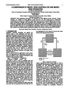
2. ACTIVE APPEARANCE MODELS An active appearance model (AAM) is a statistical model that combines shape and appearance information to form a non-rigid model of an image region. The AAM algorithm [1] describes an iterative scheme to fit this model to an example image. An AAM is built by first considering shape and appearance variation independently across a training set of images, then combining to form a single model. 2.1. Shape Modelling Shape deformations of an image region, e.g. face or lips, seen in a training set can be described using the eigenspace of a set of landmark points. The entire face is modelled using 68 points to outline the eyebrows, eyes, jaw, mouth inner and outer contour, and line down the bridge and under the nose, see figure 1.

Figure 1: Example of the 68 landmark points used for shape modelling. Landmark points were manually located in a training set of 4,072 images. Shape s, is described by the 2N -dimensional vector of N concatenated landmark (x , y) coordinates, s = [x1 , y1 , x2 , y2 ,..., xN , yN ]T .

(1)

A similarity transform (translation, rotation and scaling) is used in an iterative Procrustes analysis [1] to align each shape in the training set. This step ensures that the variation in the training set is due only to shape differences. The main modes of shape variation, i.e. axes of greatest variance, are found using PCA. Valid shape variation is compactly modelled as a projection into a subset of this eigenspace, s ≈ s + Ps bs ,

(2)

where s is the mean aligned shape, Ps is the matrix of t shape eigenvectors [ ps1 , ps2 ,..., pst ] , and bs is the t dimensional vector of corresponding weights (the principal components). The dimensionality, t is chosen so that the sum of the top t eigenvectors describes some portion of the total variance. Figure 2 shows the mean face shape deformed by projecting up to ±3 standard deviations for the first four modes. The final shape model uses 11 modes to describe 85% of the variance of the labeled training images from the IBM ViaVoiceTM database.

training examples. Shape-normalised appearance is approximated using the top t eigenvectors from PCA, a ≈ a + Pa ba ,

(3)

where Pa is the matrix of t shape normalised appearance eigenvectors, and ba is the t-dimensional vector of corresponding weights. Figure 4 shows the mean shape-normalised appearance and projections at ± 3 standard deviations for the first four modes. The shape-free appearance model uses 186 modes to describe 85% of the variance of the labelled training images from the IBM ViaVoiceTM database.

+3σ mode 1

mode 2

mode 3

mode 4

Figure 2: Statistical shape model. Each mode is plotted at ±3 standard deviations around the mean. The top four modes describe 65% of the variance of the training set.

−3σ

2.2. Shape-Free Appearance Modelling PCA can also be used to compactly model pixel intensity, or colour, variation over a training set of images, and is often called “eigenfaces” [9]. Pixel values in an N × M image are represented as a single NM -dimensional vector by sampling the image from its rows or columns. The extension to a colour image is simply to sample each colour attribute for each pixel. All appearance modelling in this paper uses colour images. A problem using this approach is that background pixels in the image can introduce significant unwanted variance. Typically, a region of interest (ROI) in the image is located to remove as much background as possible. This is the approach used in section 3. A more specific model can be obtained by sampling only the pixel values that lie within the region to be modelled, for example the face. However, this region is generally deformable and cannot be sampled reliably. One solution is to warp all training images to a reference shape before sampling. A warp is defined using the landmark points labelled for shape modelling as source vertices, and the mean shape points s, as destination vertices. The image then forms the texture map for a texture mapping operation that can be implemented using a graphics API such as OpenGL, and is usually hardware accelerated. The size of the reference shape can be chosen to define the number of appearance pixels to be modelled, 6000 in this case. Figure 3 illustrates this process. The reference shape could be arbitrary, but the mean shape is convenient.

labelled image

face region

mean

warped image

Figure 3: Appearance shape normalisation. Labelled landmark points are texture mapped to the mean reference shape. The appearance can now be sampled in this reference frame, where each pixel has approximately equivalent meaning for all

mode 1

mode 2

mode 3

mode 4

Figure 4: Shape free appearance. Centre row, mean appearance. Top and bottom row, +3 and −3 standard deviations from the mean respectively. The top four modes describe 33% of the training set variance.

2.3. Combined Shape and Appearance Model Often there is significant correlation between shape and appearance. For example, lips look different when the mouth is open and the oral cavity is seen. A third PCA can be used to decorrelate the individual shape and shape-normalised appearance eigenspaces and create a combined shape and appearance model. The combined shape and appearance space is generated by concatenating the shape and appearance model parameters into a single vector, c = [ bTs , bTa ]T . (4) As these parameters represent projections on (x , y) coordinates and pixel intensity values respectively, PCA cannot be applied directly on the combined vectors. A weighting factor is used to equalise the relative variance contribution from shape and appearance parameters. When the weighted, concatenated parameters are transformed using a final PCA the combined shape and appearance model is obtained, c ≈ Pc bc , (5) where Pc is the matrix of t combined shape and appearance eigenvectors and bc is the t-dimensional vector of weights. Figure 5 shows the top four, out of 86 modes of the final model describing 95% of the combined variance. 2.4. Fitting Small perturbations in the model parameter set, δm, are assumed to have a linear relationship to the difference between the current

+3σ

mean

−3σ mode 1

mode 2

mode 3

mode 4

Figure 5: Combined shape and appearance. Centre row, mean shape and appearance. Top and bottom row, +3 and −3 standard deviations respectively. The top four modes describe 46% of the combined variance. model projection and the image, δa = ai − a, where a is the shape-normalised image appearance, and ai is the current model appearance. For fitting, m includes pose parameters as well as combined model parameters bc . Given a training set of model perturbations δm, and corresponding difference appearances δa, a linear update model, δm = R δa ,

(6)

can be solved for R, using linear regression. The training set can be synthesised to an arbitrary size using random perturbations of the model parameters and recording the resulting difference appearance. The combined model (5) is fitted to an example image by iteratively applying the update prediction (6). Visual speech features can be directly obtained using the resulting 86 dimensional TM model parameters bc . Images in the IBM ViaVoice database are 704 × 480 pixels and were tracked at 4–5 frames per second. 3. IMAGE TRANSFORMATION FEATURES An alternative method for coding visual features is to directly transform the image pixel values around the lips into a lower dimensional space. Ideally this transform will remove redundant information and code only salient visual speech features. In practice, linear transforms provide good results and are readily implementable. Three are considered here; the discrete cosine transform (DCT), the discrete wavelet transform (DWT) and principal component analysis (PCA). The face region is automatically located in each image using the algorithm described in [6]. The lip region is then extracted using lip contour points, and scaled to 64 × 64 pixels. Pixel luminance values are sampled to form a 4096 dimensional vector. Some example faces are shown in figure 6 with corresponding mouth regions. The discrete cosine transform is similar to the discrete Fourier transform (DFT) but represents the data using only (real) cosine basis functions. The discrete wavelet transform [5] is another orthogonal, linear transform, but the basis functions are more complex and localised. Both second and third order Daubechies class wavelet filters (DWT 2 and DWT 3) are used. Full details of the implementation can be found in [3, 4].

Figure 6: Region of interest extraction. Top rows show example video frames from 8 database subjects. Lower row shows corresponding extracted mouth regions of interest.

Principal component analysis has been described in section 2.1. The only difference when applying directly to image regions is that the data are scaled according to the variance in each dimension. This normalises the feature space and accords equal importance to each dimension. This is computed by calculating the eigenvectors and eigenvalues of the correlation matrix. To simplify the PCA calculation the mouth region images were further subsampled to 32 × 32 pixels. In all cases, visual features are formed by taking the 24 highest energy components from the transform, considered over all the training data. 4. MATCHED DISCRIMINANT FEATURES All the visual front ends, AAM, DCT, DWT and PCA, are further subject to a two stage transformation to form the final visual features. The first stage uses linear discriminant analysis (LDA) to find the best linear transform to separate the feature space according to a set of classes. In this case 2808 HMM states are used to classify the data. To explicitly model dynamic visual speech information, LDA is applied to 15 temporally concatenated features. Only the top 41 features in the LDA transformed space are retained. The final step is a feature space rotation using a maximum likelihood linear transform (MLLT). MLLT considers the observation data likelihood in the feature space under the assumption of diagonal data covariance in the transformed space. Further details of the implementation can be found in [4]. The final features in all cases are 41 dimensional. 5. DATABASE AND EXPERIMENTAL RESULTS A subset of 4,952 sequences, representing 1,119,256 images, of TM the IBM ViaVoice database was used for all experiments. This covers 10 hrs, 22 mins of video data at 30 frames per second. From this 4,441 sequences are used for training data, and 506 sequences are used for test data in a speaker independent task on a 10,500 word vocabulary A further subset of 4,072 images taken from 323 sequences was used to train the AAM. This took significant effort, as each image had 68 points manually labelled, but covers only 2 mins 13 secs of video data.

The mean square pixel error between the model fit and image can be computed for each frame of the AAM tracked images. The average error over an entire sequence varies between 89.1 (best fitted) to 548.9 (worst) with a mean fit error of 254.2. Visual inspection of the results show that the AAM often failed to follow small facial motions. Visual features were compared by training visual-only HMM’s. Three state, 12 Gaussian mixture, triphone models were created using standard acoustic decision tree based clustering. The visual HMM’s were then used to rescore lattices obtained using noisy, audio-only HMM’s. The noisy audio models were obtained by training on acoustic data corrupted by additive ‘babble’ noise at 8.5 dB. Because of the rescoring methodology, the recognition results cannot be interpreted as visual-only results. These experiments are to determine whether the visual parameterisation used is able to extract useful additional speech information. Further details of the experimental setup are described in [2]. The large vocabulary, continuous, audio-visual speech recognition word error rate (WER) scores obtained for all features are summarised in table 1. The best visual results are obtained using the DCT transform-based features. The oracle result (best path through the lattice), anti-oracle (worst path), and best path using only the language model are also shown. The best overall performance was obtained using noisy acoustic (MFCC) features, similar to those used to obtain the lattice. Modality Visual

Acoustic None

Parameterisation DCT DWT 3 PCA DWT 2 AAM MFCC (noisy audio) Oracle Anti-oracle LM best path

WER % 58.1 58.8 58.8 59.4 64.0 55.0 31.2 102.6 62.0

Table 1: Speaker independent, large vocabulary, continuous, audio-visual recognition word error rates (WER) for each of the proposed visual feature parameterisations, based on lattice rescoring. Audio-only (at 8.5 dB SNR), and characteristic lattice WERs are also shown.

6. SUMMARY This paper compares four different visual speech parameterisations in a large vocabulary, continuous, audio-visual speech task. Three of these methods, DCT, DWT and PCA, are image-transform based techniques that require the ROI around the mouth to be located. The fourth, AAM, attempts to model the entire face as a deformable model of facial appearance and includes a tracking algorithm. Using the entire face improves tracking performance as the region has more appearance constraints. There is also evidence that including additional facial features will be beneficial [8, 10]. Experimental results show that the image transform methods perform better. The AAM based features suffer from the common problems of a model-based method; modelling and tracking errors. Most significant is the measurable poor tracking performance. This is a function of the extremely small amount of model

training data and the fitting algorithm. In particular, the linear regression approach to calculating model updates suffers from being undersampled for high dimensional models. The AAM features were the only ones to perform worse than using only the language model to decode the noisy audio-only lattice. By incorporating suitable prior knowledge and integrating tracking and parameterisation we hope that a more robust model-based approach may yet turn out to be a useful method. 7. ACKNOWLEDGEMENTS Many thanks to Laurel Phillips, Azad Mashari and June Sison for tedious landmark point labelling. The work described here was made possible thanks to the Workshop 2000 hosted by CLSP, Johns Hopkins University. 8. REFERENCES [1] T. F. Cootes, G. J. Edwards, and C. J. Taylor. Active appearance models. In Proc. European Conference on Computer Vision, pages 484–498, 1998. [2] C. Neti, G. Potamianos, J. Luettin, I. Matthews, H. Glotin, D. Vergyri, J. Sison, A. Mashari, and J. Zhou. Audio-visual speech recognition. Technical Report WS00AVSR, Johns Hopkins University, CLSP, 2000. [3] G. Potamianos, H. P. Graf, and E. Cosatto. An image transform approach for HMM based automatic lipreading. In Proc. IEEE International Conference on Image Processing, volume III, pages 173–177, Chicago, 1998. [4] G. Potamianos, A. Verma, C. Neti, G. Iyengar, and S. Basu. A cascade image transform for speaker independent automatic speechreading. In Proc. International Conference on Multimedia and Expo, volume II, pages 1097–1100, New York, 2000. [5] W. H. Press, S. A. Teukosky, W. T. Vetterling, and B. P. Flannery. Numerical Recipies in C: The Art of Scientific Computing. Cambridge University Press, second edition, 1995. [6] A. W. Senior. Face and feature finding for a face recognition system. In Proc. International Conference on Audio and Video-based Biometric Person Authentication, pages 154– 159, Washington, 1999. [7] D. G. Stork and M. E. Hennecke, editors. Speechreading by Humans and Machines: Models, Systems and Applications, volume 150 of NATO ASI Series F: Computer and Systems Sciences. Springer-Verlag, Berlin, 1996. [8] Q. Summerfield. Some preliminaries to a comprehensive account of audio-visual speech perception. In B. Dodd and R. Campbell, editors, Hearing by Eye: The Psychology of Lip-reading, pages 3–51. Lawrence Erlbaum Associates, London, 1987. [9] M. Turk and A. Pentland. Eigenfaces for recognition. Journal of Cognitive Neuroscience, 3(1):71–86, 1991. [10] E. Vatikiotis-Bateson, K. G. Munhall, and M. Hirayama. The dynamics of audiovisual behavior in speech. In Stork and Hennecke [7], pages 221–232. [11] S. Young, D. Kershaw, J. Odell, D. Ollason, V. Valtchev, and P. Woodland. The HTK Book. Entropic Ltd., Cambridge, 1999.