Neuro-fuzzy model and Regression model a comparison study of MRR in Electrical discharge machining of D2 tool steel M. K. Pradhan*, and C. K. Biswas,
Abstract—In the current research, neuro-fuzzy model and regression model was developed to predict Material Removal Rate in Electrical Discharge Machining process for AISI D2 tool steel with copper electrode. Extensive experiments were conducted with various levels of discharge current, pulse duration and duty cycle. The experimental data are split into two sets, one for training and the other for validation of the model. The training data were used to develop the above models and the test data, which was not used earlier to develop these models were used for validation the models. Subsequently, the models are compared. It was found that the predicted and experimental results were in good agreement and the coefficients of correlation were found to be 0.999 and 0.974 for neuro fuzzy and regression model respectively Keywords—Electrical discharge machining; Material Removal Rate; Neuro-fuzzy model; Regression model; Mountain clustering.
I. I NTRODUCTION
T
Here is a heavy demand of the advanced materials with high strength, high hardness, temperature resistance and high strength to weight ratio in the present day technologically advanced industries like, an automobile, aeronautics, nuclear, mould tool and die making industries etc. This need leads to evolution of advance materials like high strength alloys, ceramics, fiber-reinforced composites etc. While machining these materials, traditional manufacturing processes are increasingly being replaced by more advanced techniques which use different form of energy to remove the material because these advance materials are difficult to machine by the conventional machining processes, and it is difficult to achieve good surface finish and close tolerance. With the advancement of automation technology, manufacturers are more interested in the processing and miniaturization of components made by these costly and hard materials. EDM has grown over the last few decades from a novelty to a mainstream manufacturing process. It is most widely and successfully applied for the machining of various work piece materials in the said advance industry[1]. It is a thermal process with a complex metal removal mechanism, involving the formation of a plasma channel between the tool and work piece electrodes, the repetitive spark cause melting and even evaporating the electrodes. In M. K. Pradhan is Research Scholar, Department of Mechanical Engineering, National Institute of Technology, Rourkela, India e-mail:
[email protected]. C. K. Biswas is Assistant Professor and head of the manufacturing engineering Laboratory in the department of Mechanical Engineering, N.I.T, Rourkela, India. Click:- http://www.waset.org/journals/ijmpes/v3/v3-1-8.pdf
the recent years, this technology has firmly established for the production of tool to produce die-castings, plastics and moulding, forging dies etc. The advantage of this process is its capability to machine difficult to machine materials with desired shape and size with a required dimensional accuracy and productivity. Due to this benefit, EDM is a widespread technique used in modern manufacturing industry to produce high-precision machining of all types of conductive materials, alloy’s and even ceramic materials, of any hardness and shape, which would have been difficult to manufacture by conventional machining. Significant developments have been carried out in the process of EDM to increase the productivity and accuracy to increase the versatility of the process. The important concern is the optimization of the process parameters such as pulse current intensity (Ip), pulse duration (Ton), duty cycle 𝜏 and open-circuit voltage (V) for improving MRR simultaneously minimize the tool wear and Surface roughness. Several researches have been carried out for predictive modeling to increase the productivity i.e. MRR and are reported in the literature [2]. In recent years, many attempts have been made for modeling the EDM process and investigation of the process performance to recuperate MRR [3]-[4]. Improving the MRR and surface quality are still challenging problems that restrict the expanded application of the technology [5]. Semi-empirical models of MRR for various work piece and tool electrode combinations have been presented by Wang and Tsai [6]. To achieve high removal rate in EDM, a stable machining process is required, which is partly influenced by the contamination of the gap between the workpiece (hardened steel 210CR12) and the electrode, and it also depends on the size of the eroding surface in the given machining regime [4]. In recent times, Artificial Neural Networks (ANNs) and fuzzy logic have emerged as a highly flexible modeling tool for manufacturing sectors. As far as EDM is concerned, the relative literature includes publications where ANNs are applied, mainly, for the estimation or prediction of the MRR, the optimization and the on-line monitoring of the process. Tsai and Wang have compared the six different neural networks together with a neuro-fuzzy network models on MRR and reported that adaptive-network fuzzy interference system (ANFIS) shows the accurate results [7]. ANFIS is a fuzzy inference system implemented in the framework of neural networks. Wang et al. [?] use hybrid model of ANN and Genetic Algorithm and found that the error of the model is 5.6% for MRR. Panda and Bhoi [8] to predict MRR using feed forward ANN based on the
Levenberg-Marquardt back propagation technique. Pradhan et el. [9] compared two neural network models namely back propagation and radial basis function for the prediction of surface roughness on AISI D2 steel and concluded that radial basis function models reasonably more accurately. Currently, a new trend has been introduced to combine the features of two or more than two techniques to exploit the potential of each technique and diminish their disadvantages. Such technique with combined features is called as hybrid modeling technique. Presently, the neuro-fuzzy approach is becoming one of the major areas of interest because it gets the benefits of neural networks as well as of fuzzy logic systems, and it removes the individual disadvantages by combining them on the common features. However, several works had been carried out on prediction of MRR of various workpiece materials in EDM process, but no reported literature has referred to the modeling of MRR of AISI D2 steel using the neuro-fuzzy system. In the present study, a neuro-fuzzy model is developed to predict MRR of EDMed AISI D2 steel. The proposed models use data for training procedure from an extensive experimental research concerning EDM. The Ip, Ton and 𝜏 were considered as the input parameters of the models. The Ip, Ton and 𝜏 varied over a wide range, from roughing to near-finishing conditions keeping Voltage (V) constant. The training data set is used to obtain fuzzy rules using the mountain clustering technique and rules are fine tuned using the back propagation algorithm. After validation of the model, total data are forwarded for prediction of MRR. A nonlinear regression model is also obtained from same data for comparison with the present model. The proposed neuro-fuzzy network is proven successful, resulting in reliable predictions, providing a possible way to avoid time and money-consuming experiments. II. EXPERIMENTATION A number of experiments were conducted to study the effects of various machining parameters on EDM process. These studies have been undertaken to investigate the effects of Ip, voltage (V), Ton and duty cycle on MRR. Where, duty cycle is defined as
workpiece materials used were AISI D2 steel square plates of surface dimensions 1515 mm2 and of thickness 4 mm. Commercial grade EDM oil (specific gravity= 0.763, freezing point= 94?C) was used as dielectric fluid. Lateral flushing with a pressure of 0.3 kgf/cm2 was used. The test conditions are depicted in the Table 2. To obtain a more accurate result, each combination of experiments (90 runs) was repeated three times and every test ran for 15 min. TABLE I C HEMICAL COMPOSITION OF AISI D2 ( WT %)
Cr 11.5
Mo 0.70
V 1.00
C 1.55
(1)
The selected workpiece material the research work is AISI D2 (DIN 1.2379) tool steel. The chemical composition of work material is mentioned in Table-1. The workpiece material D2 steel, which is an air hardening, high carbon, high chromium tool steel possessing extremely wear resisting properties and is practically free from size change after proper treatment. It is selected due to its growing range of applications in the field of manufacturing tools in mold making industries. The electrode material for these experiments is copper. Experiments were conducted on Electronica Electraplus PS 50ZNC die sinking machine. A cylindrical pure copper, with a diameter of 30 mm, was used as a tool electrode (of positive polarity) and
Si 0.25
Ni 0.3
Fe Balance
TABLE II E XPERIMENTAL CONDITIONS
Sparking voltage in V Current (Ip), in A Pulse on Time (Ton), in 𝜇s Duty Cycle (𝜏 ) Dielectric used Dielectric flushing Work material Electrode material Electrode polarity Work material polarity
50 10 20 30 50 100 150 200 500 750 1 6 12 Commercial grade EDM oil Side flushing with pressure AISI D2 steel Electrolytic pure Copper Positive Negative
A. Calculation of MRR The calculations of the workpiece material removal rate (MRR) were based on the measurement of weight loss, and the change in weight was converted to the change in volume. The weight loss was measured by an electronic balance with a readability of 1 mg. The MRR were calculated by using the volume loss from the workpiece divided by the time of machining.
𝑀 𝑅𝑅 = 𝑇 𝑜𝑛 × 100 𝐷𝑢𝑡𝑦 𝐶𝑦𝑐𝑙𝑒 = 𝑇 𝑜𝑛 + 𝑇 𝑜𝑓 𝑓
Mn 0.30
Δ𝑉𝑤 Δ𝑊𝑤 = 𝑇 𝜌𝑤 𝑇
(2)
Where Δ𝑉𝑤 is the volume loss from the work piece, Δ𝑊𝑤 is the weight loss from the work piece, T is the duration of the machining process, and 𝜌𝑤 = 7700 𝑘𝑔/𝑚3 the density of the work piece. III. PREDICTIVE MODELS FOR MRR A. Regression models Based on the experimental data gathered, statistical regression analysis enabled to study the correlation of process parameters with the MRR. Both linear and non-linear regression models were examined; acceptance was based on high to very high coefficients of correlation (r) calculated. In this study, for three variables under consideration, a polynomial regression is
used for modeling. For simplicity, a quadratic model of MRR is proposed and can be written as shown in Equation 3. The coefficients of regression model can be estimated from the experimental results. The effects of these variables and the interaction between them were included in this analyses and the developed model is expressed as interaction equation: 𝑀 𝑅𝑅 = 𝑎0 + 𝑎1 𝐼𝑝 + 𝑎2 ln(𝑇 𝑜𝑛) + 𝑎3 𝜏 + 𝑏1 (𝐼𝑝)2 +𝑏2 (ln(𝑇 𝑜𝑛))2 + 𝑏3 (𝜏 )2 + 𝑐1 𝐼𝑝 ln(𝑇 𝑜𝑛) +𝑐2 ln(𝑇 𝑜𝑛)𝜏 + 𝑐3 𝐼𝑝𝜏 + 𝑑1 𝐼𝑝 ln(𝑇 𝑜𝑛)𝜏
(3)
Where 𝑎0 is the free term, and 𝑎1 , 𝑎2 and 𝑎3 are the linear effects. The regression analysis shows that the possible relationship between MRR and Ip, Ton and 𝜏 are the following: The coefficient 𝑎0 is the free term, the coefficients 𝑎𝑖 are the linear terms, the coefficients 𝑏𝑖 are the quadratic terms, and the coefficients 𝑐𝑖 and 𝑑𝑖 are the interaction terms. The regression analysis showed that the possible relationship between MRR and Ip, Ton and 𝜏 are the following, 𝑀 𝑅𝑅
= +
−3.9064 + 0.442𝐼𝑝 − 0.08286 ln(𝑇 𝑜𝑛) 0.7645𝜏 + 0.00068(𝐼𝑝)2 + 0.11062(ln(𝑇 𝑜𝑛))2
− +
0.098(𝜏 )2 − 0.029𝐼𝑝 ln(𝑇 𝑜𝑛) − 0.005 ln(𝑇 𝑜𝑛)𝜏 0.06𝐼𝑝𝜏 + 0.0315𝐼𝑝 ln(𝑇 𝑜𝑛)𝜏 (4)
to clustering using Mountain clustering technique [10]. The stopping constant of 0.001, mountain building and destruction constants of 2 and 5, respectively were considered. These yield 190 rules to predict MRR, which were subsequently fine tuned by Back-propagation technique [11]. Each variable was fuzzified with ten Gaussian membership classes, without any prejudice. The error signal between the inferred output value and the respective desired value is used by the gradientdescent method to adjust each rule conclusion with learning rate of 0.0001 and maximum of 105 epochs. Since, Gaussian membership function is associated with product composition for ease in calculation, we have used the same. Lastly, the inference mechanism weights each rule value were defuzzified by centriod method. The RMS error for validation data set was calculated for each epoch and the learning continued till the RMS error was found to decrease after each epoch. This inhibited the rule base to be over trained for the training data set, otherwise it may cause increase in RMS error in the validation data set.
This equation is used for the prediction of MRR for nonlinear model. B. Neuro-fuzzy models Recently, researchers are working on combining the features of two or more than two techniques to exploit the potential of each technique and diminish their disadvantages. For this they used neural network, fuzzy logic, neuro-fuzzy, ANFIS, etc. The motivation for hybridization is the technique enhancement factor, multiplicity of application tasks and realizing multifunctionality. The need for replacing these primary functions is to increase the execution speed and enhance reliability. A highly complex and ill-defined mathematical system can be modeled with neuro-fuzzy system. A neuro-fuzzy logic system contains four major components: fuzzifier, inference engine, rule base, and defuzzifier. The system can extract knowledge in form of interpretable fuzzy linguistic rules, i.e., rules that can be expressed as: If x is A and y is B then output belongs to class C. The system identifies the membership level of an input pattern to the different available membership classes and estimates the output associated with the physical phenomena. This paper proposed the neurofuzzy inference system with three input variables (discharge current, spark on-time and duty cycle) and one output variable (MRR). The experimental data are divided into training set and validation set. The former is used to extract the rules base for further validation. The neuro-fuzzy scheme is shown is Fig. 1. Layer 1 consists of fuzzification of input parameters; and the inference engine and rule base are depicted as layer 2. In the third layer, the output is defuzzified to estimate a crisp output value. The input-output training data are subjected
Fig. 1.
Three layer structure of Neuro fuzzy system
IV. RESULT AND DISCUSSION The experiments were conducted and the impact of the machining parameters such as Ip, Ton and 𝜏 on MRR is analyzed. MRR is convincingly dependent of spark energy, which is crossing the discharge gap, instigate melting of the material. The spark input energy is dependent on discharge voltage, Ip and Ton [12]. The MRR is predicted by regression model, and neuro fuzzy model. The effects of each of parameter on MRR are compared with different models and discussed. As expected, MRR is found to be increase sharply with the increase in Ip (Fig. 2), at Ton 10 𝜇s and voltage 50 volt. It is expected, because with the increase in the Ip, the spark energy increases. Thus the amount of heat going to the workpiece is more, which is responsible to increase the temperature at the nodes in the workpiece domain. Hence, volume of material having temperature above the melting temperature of workpiece is also increased. It increases the amount of material removed from the workpiece. Since, the duty cycle is the ratio of Ton to pulse period (sum of Ton and Toff as given in Equation 1), for a constant Ton, higher the 𝜏 , lower will be the Toff and vice versa. When 𝜏 decreases, the Toff is more and as a consequence, there will be an undesirable heat loss that does not contribute to MRR.
15.5
Ton = 10 µs 13.0
τ =12
MRR (mm 3/min)
10.5 τ=6 8.0
5.5
τ =1 3.0
0.5
5
Fig. 2.
6
7
8
Ip (A)
9
10
Effect of discharge current on MRR for various duty cycles
This will lead to drop in the temperature of the workpiece before the next spark starts and therefore, MRR decreases. In other words, the highest temperature goes on increasing with increase in 𝜏 . The reason is again same that with the increase in 𝜏 there is increase in Ton and correspondingly in MRR also.
τ =12
Ip=10 A
Expt. Neuro fuzzy Regression
25
20
MRR (mm 3/min)
τ=6
15
The effect of Ton and 𝜏 on MRR is shown in Fig. 3, which shows the comparison of MRR computed by the regression model, and neuro-fuzzy models, and the experimental results for various Ton with constant voltage = 50 volt and Ip=10A. It can be inferred that MRR increases when the Ton increases to an optimum value and thereafter start to decrease slightly or remains constant. This is due to the fact that although spark energy increases with increasing Ton, however, the present trend of MRR at higher Ton is due to insufficient flushing and arcing phenomena, which is more prominent while machining with higher Ton. This also depicts how accurately the neurofuzzy model predicts the MRR and When increase from 1 to 6 there is a sharp increase in MRR as compared to the increase in MRR from = 6 to 12. To show the highest accuracy of the neuro-fuzzy model, some graphs were plotted. Fig. 4, present plots of the experimental MRR versus the predicted values obtained using the said models neuro-fuzzy and regression model. These plots also present straight lines to make them easier to interpret. The figures shows that models could predict very accurately and except for one or two outliner, almost all the values are very close to the line. It could be noted that closer the value to the line, more is the accuracy. The represented data refer to both the training and the validation data sets. These representations show how the fuzzy model is better in accuracy than the regression model confirming the effectiveness of the neuro-fuzzy approach to the proposed problem. It is conformed by the correlation co-efficient between predicted MRR and experimental MRR as 0.991 and 0.999 for the regression and neuro-fuzzy, respectively. Fig. 5 both the models are depicted in the same figures, it can be observed that the models provides similar results at the higher value of MRR, however at lower MRR, they diverse a little from each other.
10
τ =1
40
0
Fig. 3.
50
100
Ton ( µs)
150
200
Effect of Ton on MRR with various duty cycles
Predicted MRR (mm 3/min)
5
30
20
10
Neuro fuzzy Model
Regression Model
Predicted MRR (mm 3/min)
Predicted MRR (mm 3/min)
0
30
20
10
0
0
10
20
30
Expt. MRR (mm 3/min)
5
10
15
20
25
30
35
40
Expt MRR (mm 3/min)
20
Fig. 5. Comparison predicted (Neuro-Fuzzy model and Regression model) and experimental results 10
0
0
Fig. 4.
30
0
10
20
30
Expt. MRR (mm 3/min)
Comparison predicted and experimental results
Residuals obtained are plotted against run for both the models and shown in Fig. 6. It shows the residuals for regression and neuro-fuzzy model, calculated as the difference between the measured and the predicted values of the MRR. These residuals which are very large or very small than the rest are typically called Outlier and a few such outliners may
Mean 0.2061 StDev 2.675 N 46
20
3
2
Frequency
15
Residuals
1
0
10
5
-1
-2
0
Neuro fuzzy Regression
-3
0
5
10
15
20
25
30
35
40
MRR (mm 3/min)
-8
-4 0 Residues (Regression)
4
8
Histogram plot of residuals (Regression model)
Residuals verse predicted MRR for all runs
distort the analysis. The residuals of the regression and NF are very close to zero and exhibit randomness with run without any outliners. It is found that the residuals are between -0.98 to 1.55, and -3.58 to 3.49 for neuro-fuzzy, regression predictive modeling respectively for training data. And, similarly for testing data set, the residues are -1.3 to 1.34, and -11.35 to 7.06 for neuro-fuzzy and regression predictive models, respectively. As indicated by the residues, the neuro-fuzzy model has the least residue, so the better is the prediction of the physical phenomena.
no pattern. A poorly fitted model may exhibit an increase and then decrease in the residual values with increase in the fitted value. Due to lack of fit, one or more outliners may exist, which appear as points that are either much higher or lower than normal residual value. Expt Regression Neuro Fuzzy 30
MRR (mm 3/min)
Fig. 6.
Fig. 8.
-12
12 10
20
10 Mean 0.3230 StDev 0.7045 N 46
Frequency
0
8 0
6
Fig. 9.
2
Fig. 7.
20
30
40
Expt No
4
0
10
-1.2
-0.6
-0.0 0.6 Residues (Neuro fuzzy)
1.2
1.8
Histogram plot of residuals (Neuro fuzzy model)
The deviations in predictions of MRR from the experimental results are presented in the form of histogram plots in Fig. 7, and Fig. 8 for NF and regression models, respectively. If the normality assumption of the residuals is valid, a histogram plot of the residuals should look like a sample form a normal distribution. It can be seen that both the models the distribution is the Gaussian distribution. However one or two Outliers exists in the regression model. In addition the range of MF model is -1.2 to 1.8 and that of regression model is -12 to 8. Residual analysis is standard part of assessing model adequacy at any time of mathematical model is generated because residuals are the best estimate of error. For a good model fit, this plot should show a random scatter and have
Comparisons of experimental and predicted MRRs with Expt. No
The experimental results of MRR and the predicted values regression and NF models as shown in Fig. 9 with increasing MRR, The NF models is able to follow the trend very accurately, however regression model, accept three Outliers are sufficiently close to experimental data for training and validation sets. Conclusively speaking, the NF and regression models are capable of predicting the MRR with reasonable accuracy within the experimental domain. However the neurofuzzy model shown better predictions capability than the regression model. The validations of both the models are performed with the testing data sets that are not earlier used to develop the model. In order to estimate the accuracy of the prediction models, percentage error and average percentage error are used. Prediction error has been defined as follows ∣𝐸𝑥𝑝𝑡. 𝑀 𝑅𝑅 − 𝐹 𝑖𝑡𝑡𝑒𝑑 𝑀 𝑅𝑅∣ × 100 𝐸𝑥𝑝𝑡. 𝑀 𝑅𝑅 (5) In Table III, the process parameters of testing data, their
𝑃 𝑟𝑒𝑑𝑖𝑐𝑡𝑖𝑜𝑛 𝑒𝑟𝑟𝑜𝑟 =
TABLE III C OMPARISON OF EXPERIMENTAL RESULTS WITH THE MODEL PREDICTION
Expt No 1 2 3 4 5 6 7 8 9 10
Ip (A) 15 5 10 10 10 20 20 20 20 30
Ton (𝜇s) 100 100 50 100 100 100 100 150 500 200
𝜏 12 6 6 1 12 1 6 1 1 1
Expt Pred. Residue MRR MRR NF NF 5.17 5.62 0.45 5.70 5.87 0.18 13.34 13.39 0.05 5.71 5.86 0.14 21.66 22.03 0.37 12.05 11.91 -0.14 37.12 35.98 -1.14 10.94 10.75 -0.18 10.47 10.22 -0.25 17.09 17.12 0.03 Average prediction error (%)
corresponding experimental MRR, percentage error and the average percentage error are shown. I could be noted that the maximum prediction errors are ranging from −1.19% to 8.76 and −27.93% to 23.48% for NF, and regression models, respectively. The average percentage error of these model validations are about 2.49% and 15.62 % for NF and regression model, respectively. V. C ONCLUSION This paper proposes a hybrid intelligent technique namely, neuro-fuzzy model and a regression model for the prediction of MRR of EDM. The MRR increase with the increase in discharge current and there is a sharp increase in MRR at a lower duty cycle in comparison to at a higher duty cycle; while with the increase in spark on-time the MRR increases and reaches to a maximum value and then starts to decrease. The predictions are validated with the experimental results and found to be in very good agreement. Comparisons are also made among the predicted results of the neuro-fuzzy system with regression models and establishing the superiority of the proposed model. The predictions are validated with the experimental results and compared with the regression model. Neuro-fuzzy model is found to be in very good agreement with the experimental results with average prediction error of 2.49% for validation set. The proposed network has proven to be successfully model EDM process, resulting in reliable predictions, and providing a possible way to avoid time and money-consuming experiments. R EFERENCES [1] R. Snoeys, F. Staelens, and W. Dekeyser, “Current trends in nonconventional material removal processes,” Ann. CIRP, vol. 35(2), p. 467 480, 1986. [2] K. H. Ho and S. T. Newman, “State of the art electrical discharge machining (edm),” International Journal of Machine Tools and Manufacture, vol. 43, pp. 1287–1300, Oct 2003. [3] K. Wang, H. L. Gelgele, Y. Wang, Q. Yuan, and M. Fang, “A hybrid intelligent method for modelling the edm process,” International Journal of Machine Tools and Manufacture, vol. 43, pp. 995–999, Aug 2003. [4] G. V. C.J. Luis, I. Puertas ., “Material removal rate and electrode wear study on the EDM of silicon carbide,” Journal of Materials Processing Technology, vol. 164-165, pp. 889–896, 2005.
% error NF 8.76 3.09 0.36 2.51 1.70 1.19 3.06 1.67 2.40 0.19 2.49%
Pred. MRR Reg. 6.612 6.666 12.74 3.893 20.455 9.226 30.05 9.638 11.07 15.43
Residue Reg. -1.44 -0.97 0.59 1.82 1.11 2.83 7.06 1.30 -0.61 1.65
%error Reg. 27.93 17.04 4.414 31.86 5.120 23.44 19.01 11.85 5.837 9.666 15.62 %
[5] J. Valentincic and M. Junkar, “On-line selection of rough machining parameters,” Journal of Materials Processing Technology, vol. 149, pp. 256–262, Jun 2004. [6] P. Wang and K. Tsai, “Semi-empirical model on work removal and tool wear in electrical discharge machining,” Journal of Materials Processing Technology, vol. 114, no. 1, pp. 1–17, 2001, cited By (since 1996): 11. [7] K.-M. Tsai and P.-J. Wang, “Predictions on surface finish in electrical discharge machining based upon neural network models,” International Journal of Machine Tools and Manufacture, vol. 41, pp. 1385–1403, Aug 2001. [8] D. K. Panda and R. K. Bhoi, “Artificial neural network prediction of material removal rate in electro- discharge machining,” Materials and Manufacturing Processes, vol. 20, pp. 645–672., 2005. [9] M. K. Pradhan, R. Das, and C. K. Biswas, “Comparisons of neural network models on surface roughness in electrical discharge machining,” Proceedings of the Institution of Mechanical Engineers, Part B: Journal of Engineering Manufacture, vol. 223, p. Inpress, 2009. [10] R. Yager and D. Filev, “Approximate clustering by the mountain clustering,,” IEEE Transactions on Systems Man and Cybernetics,, vol. 24,, pp. 338–358., 1994. [11] ——, Essentials of Fuzzy Modeling and Control. New York: John Wiley & Sons, Inc, 1995. [12] D. D. Dibitono, P. T. Eubank, M. R. Patel, and M. A. Barrufet, “Theoretical model of the electrical discharge machining process i. a simple cathode erosion model,,” Journal of Applied Physics,, vol. 66, pp. 4095–4103, 1989. M K Pradhan is a Research Scholar at Dept. of Mech. Engg., N.I.T, Rourkela, India. He received his ME degree from the N. I. T, Rourkela in Production Engineering in the year 1999. He has 10 years of teaching and research experience. His area of research interest includes modeling and analysis of manufacturing processes, and optimisation. He has published more than 10 research papers in the international journal/conferences. He is life member of ISTE, IACSIT and IE (I).
Dr. C K Biswas received his M Tech and PhD degrees from the Indian Institute of Technology, Kharagpur. He has published over 5 articles in international journals and presented over 10 articles at different international conferences. Currently Dr. Biswas is an assistant professor and a head of the manufacturing engineering Laboratory in the department of Mechanical Engineering, N.I.T, Rourkela, India. He is life member of IE (I).