[20] I. H. Witten and E. Frank, Data Mining: Practical machine learning tools and ... [23] P. Baldi, S. Brunak, Y. Chauvin, C. Andersen, and H. Nielsen, âAssessing.
Proceedings of the 2007 IEEE Symposium on Computational Intelligence in Bioinformatics and Computational Biology (CIBCB 2007) 1
A Comparison of Sequence Kernels for Localization Prediction of Transmembrane Proteins Stefan Maetschke, Marcus Gallagher and Mikael Bod´en School of Information Technology and Electrical Engineering, The University of Queensland, Brisbane, Queensland 4072, Australia {stefan,marcusg,mikael}@itee.uq.edu.au
Abstract— We applied Support Vector Machines to the prediction of the subcellular localization of transmembrane proteins, and compared the performance of different sequence kernels on this task. More specifically we measured prediction accuracy, computation time, number of kernel evaluations and number of support vectors for the Spectrum, the full Spectrum, the Wildcard, the Mismatch, the Local-alignment and the Residuecoupling kernel. The Local-alignment achieved the highest prediction accuracy, with an Matthews correlation coefficient of 0.51, closely followed by the Mismatch kernel. However, the Localalignment kernel was also the most time consuming kernel and seven times slower than the Mismatch kernel. The Spectrum kernel was the fastest kernel but linked to the highest number of support vectors and kernel evaluations. The Residuecoupling kernel showed the lowest number of support vectors and kernel evaluations. No correlation between the number of support vectors and prediction accuracy could be observed. A localization predictor (TMPLoc) has been made available at http://pprowler.itee.uq.edu.au/TMPLoc.
We focus our study on localization prediction of transmembrane proteins for organelles along the secretory pathway, utilizing data of the recently published LOCATE database [9]. In the following sections we provide background material concerning the biological application, current prediction algorithms and kernel methods. A. Biological background Cells of eukaryotes are divided into several functionally and structurally different membrane-bound organelles, that are essential for the metabolism of the cell. A highly specialized transport and sorting machinery is required to distribute proteins between these locations. The transport follows mainly the secretory and endocytic pathways, that comprise the following organelles: endoplasmic reticulum, Golgi apparatus, endosome, lysosome and plasma membrane [10] (see Fig. 1).
I. I NTRODUCTION Tn contrast to soluble proteins, which reside in the cytosol or lumen of compartments, transmembrane proteins are inserted into the membranes of organelles. They perform a variety of essential functions as channels, pumps, receptors, and energy transducers, and are therefore a major target for drug development [1]. It is estimated that about 20%-30% of a proteome are transmembrane proteins [2] but structure and function are identified only for a fraction of them [3]. Determining the subcellular localization of a protein is a first step in revealing its function. The vast majority of current prediction algorithms however, are designed for soluble or prokaryotic proteins1 and achieve low accuracies when applied to transmembrane proteins in eukaryotes. Inspired by the success of the recently developed string and sequence kernels for support vector machines, we were interested in the performance of these kernels for subcellular localization prediction of transmembrane proteins. More specifically we examine the Spectrum kernel [4], a variant of the Spectrum kernel named full Spectrum kernel, the Wildcard kernel [5], the Mismatch [6], the Local-alignment kernel [7] and the Residue-coupling kernel [8] with respect to prediction accuracy, computation time, number of kernel evaluations and number of support vectors. 1 Note that the number of localizations in prokaryotes is much more limited than in eukaryotes. For instance, in Gram-negative bacteria the typical locations predicted are the inner and outer membrane only.
1-4244-0710-9/07/$20.00 ©2007 IEEE
Fig. 1.
Flow diagram of secretory, endocytic and retrieval pathways.
The secretory pathway controls the flow of newly synthesised proteins from the cell interior to all organelles along the path to the cell exterior. The reversed direction of transport, where proteins are internalized from the outside of the cell, is called the endocytic pathway. Retrieval pathways transport escaped proteins back to their original target location. Proteins can be mediated to the interior of an organelle (soluble proteins) or bound to the membrane of a compartment
367
Proceedings of the 2007 IEEE Symposium on Computational Intelligence in Bioinformatics and Computational Biology (CIBCB 2007) 2
(membrane proteins). The most common class of membrane proteins are α-helical transmembrane proteins, that are inserted into the membrane. The membrane spanning regions form α-helices and the protein can pass through the membrane once or multiple times (see Fig. 2).
Fig. 2. Single- and multi-spanning transmembrane proteins inserted into the membrane.
B. Prediction algorithms The early observation of Nakashima and Nishikawa [11], that the overall amino acid composition differs significantly between proteins of different subcellular localizations, has inspired the development of a multitude of prediction algorithms. Since our focus is on kernel methods, we will discuss only related approaches. So far only one method by Chou et al. [12] has been published that specifically predicts the subcellular localization of transmembrane proteins in eukaryotes. All other methods target soluble or prokaryotic proteins. SubLoc [13] is a predictor that calculates the amino acid composition of a sequence and employs a support vector machine with an Radial Basis Function (RBF) kernel to assign subcellular localizations to soluble prokaryotic and eukaryotic proteins. PLOC [14] is composed of 12 support vector machines and uses a jury decision to discriminate between 12 subcellular locations. The input features are the single and the pair amino acid composition and the best result was achieved with an RBF-kernel. Esub8 [15] utilizes a support vector machine with an RBFkernel and tries to take the order of sequence residues into account by splitting the sequence in two halves and calculating the amino acid composition for the first and the second part of the proteins. The CELLO software [16] characterizes proteins by four different amino acid compositions: single amino acids, amino acid pairs, amino acid triplets over a sub-alphabet and compositions for sections of the sequence. The system consists of 40 support vector machines, using RBF kernels, and predicts locations in Gram-negative bacteria only. An interesting approach has been taken by Nair and Rost with the LOCtree system [17]. In this model the architecture of the sorting machinery is mimicked by a binary decision tree where each node is a support vector machine that controls the path of a sequence through the tree. The branches of the tree represent intermediate stages in the sorting process
while the nodes are emulations of the decision points in the sorting machinery. The best performance was achieved with RBF kernels. Guo [8] introduced the residue-coupling model that encodes a sequence by compositions of gapped amino acids pairs over a range of gap sizes. This approach achieved very high prediction accuracies (88.9% on a eukaryotic dataset), utilizing support vector machines with RBF kernels. Matsuda et al. [18] split the amino acid sequence into N-terminal, middle and C-terminal part and calculated the amino acid composition, the pair amino acid composition and a frequency distribution over distances between amino acids with similar physicochemical properties (basic, hydrophobic and other) to represent a protein. They applied support vector machines with RBF kernels and reported prediction accuracies similar to Guo’s approach. The only predictor for eukaryotic membrane proteins that we are aware of is based on amino acid composition and employs a least Mahalanobis distance classifier [12]. In this paper Chou et al. extracted a data set with 2105 membrane proteins localized at nine different organelles from SwissProt (Release 35.0) and reported an overall jackknife accuracy of 65.9%. Since the data set was only weakly redundancyreduced and contained different proteins types and subcellular locations, these results are not comparable with ours. We compiled a recent, strictly redundancy reduced data set of five locations, that contains transmembrane proteins only. C. Kernel methods The classical way to represent data for machine learning algorithms is as a feature vector. For instance, an amino acid sequence can be described by a vector of its amino acid frequencies. This approach forces sequences to be encoded by a fixed number of features, even if the sequences are of variable length. Kernel methods circumvent this problem by representing data through a set of pairwise comparisons. More precisely, the mapping φ : X → F of sequences x ∈ X into a feature space F is replaced by a kernel function k : X × X → �. A data set S = (x1 , . . . , xn ) is then represented as a n×n matrix of pairwise comparisons kij = k(xi , xj ) [19]. Efficient and successful instantiations of kernel methods are Support Vector Machines (SVMs). Let (y1 , . . . , yn ), with y ∈ {−1, +1}, be a set of class labels associated with samples (x1 , . . . , xn ) in S, then SVMs utilize the following decision function f to classify a query sample x: � � n � αi yi k(xi , x) + b . (1) f (x) = sgn i=1
Equation 1 defines a hyperplane in kernel space, that is optimized by the training algorithm to separate the samples of the two classes. For a query sample x, f (x) returns +1 or −1 to indicate the class the sample is predicted to belong to. The offset b and the Lagrange multipliers αi are parameters of the hyperplane that are computed during the training of the SVM. Note that only samples xi with αi �= 0 contribute to the classification. These samples are called support vectors. To
368
Proceedings of the 2007 IEEE Symposium on Computational Intelligence in Bioinformatics and Computational Biology (CIBCB 2007) 3
train SVMs highly efficient algorithms have been developed that solve a quadratic, constrained maximization problem: n n n � 1 �� W (α) = − yi yj αi αj k(xi , xj ) + αi 2 i=1 j=1 i=1 �� (2) n i=1 yi αi = 0 subject to 0 ≥ αi ≥ C for i = 1, . . . , n. Apart from the kernel and its parameters the only user parameter of the algorithm is the complexity parameter C, that regulates the trade-off between the complexity of the classification boundary and the misclassification error. SVMs are binary classifiers by nature. Multi-class problems are typically solved by reformulating them as multiple binary classification problems and training a set of binary SVMs in a one-versus-one or one-versus-rest scheme [19]. II. M ETHODS In this section we provide details of the SVM employed, introduce the kernels examined and describe the data set that our experiments were based on. A. Support Vector Machine For all experiments we utilized the SVM algorithm of the WEKA library [20], that implements Platt’s Sequential Minimal Optimization (SMO) [21] with an improvement by Keerthi [22]. We extended the SVM implementation in WEKA to allow for arbitrary kernel functions and added caching of the kernel matrix. Following Sch¨olkopf et al. [19] the kernel matrix was normalized with kij � = � . (3) kij kii kjj Multi-class problems are solved with a one-versus-one approach in WEKA. For the five class problem (described below), ten binary classifiers are therefore created, trained and tested. The reported kernel evaluation times, number of kernel evaluations and number of support vectors were calculated as the sum over all ten binary classifiers. The prediction performance of the classifier was measured by the Matthews correlation coefficient (MCC) – a variant of the classical Pearsons correlation coefficient for discrete data [23], that is frequently used in the context of subcellular localization prediction. The MCC is defined as tp · tn − f p · f n (4) MCC = � (tp + f n)(tp + f p)(tn + f p)(tn + f n) with tp is the number of true positives, f p is the number of false positives, tn is the number of true negatives and f n is the number of false negatives. An MCC of +1 indicates perfect correlation, an MCC of −1 perfect anti-correlation and an MCC of zero no correlation at all. To assess the significance of differences in prediction performance we also report the 95% confidence interval for the MCC: σmcc (5) δ95 = ±1.96 · √ n with σmcc is the standard deviation of the MCC and n is the number of folds of the cross-validation test.
B. Kernels In this section we introduce the sequence kernels utilized in this study. We use the following terminology: A protein sequence s is described as string of symbols drawn from a 20letter amino acid alphabet A. A section of l consecutive amino acids in the sequence is called an l-mer and the amino acid composition of a sequence is the frequency distribution over the symbols of the sequence. Kernel parameters are denoted in parentheses. Spectrum(l): The spectrum is a vector over all possible lmers that can be generated from the symbols in A. It contains the frequencies of the l-mers contained in sequence s. The kernel function is defined as the dot product between the spectra of two sequences [4]. The kernel value is large if two sequences share a large number of l-mers. Note that the kernel function can be computed very efficiently due to the increasing sparseness of longer l-mers. Full-Spectrum(l): An obvious extension of the Spectrum kernel is a full Spectrum kernel that is composed of spectra with l-mer of increasing length. In contrast to the Spectrum kernel it contains not only l-mers for one specific choice of l but all l-mers from one up to l. Apart from this difference the full spectrum is calculated exactly the same way as the spectrum. Wildcard(l, m): The Wildcard kernel [5] is also an extension of the Spectrum kernel. The amino acid alphabet A is augmented by a wildcard symbol ∗ that can match any amino acid. The wildcard spectrum of a sequence is then a vector over all possible l-mers that can be drawn from A ∪ ∗ and contains at most m wildcard symbols. The kernel function is computed as the dot product of two wildcard spectra. For m = 0 the Wildcard kernel is identical to the Spectrum kernel. Note that the mismatches within an l-mer are position specific when two l-mers are compared for counting. Mismatch(l, m): The Mismatch kernel [6] can be seen as an extension of the Wildcard kernel that lifts the limitation to position specific mismatches within the l-mers. The mismatch spectrum of a sequence is a vector where each element contains the frequency of a specific l-mer and all other lmers with no more than m mismatches. The kernel output is calculated as the dot product of the mismatch spectra. Note that for m = 0 the Mismatch kernel, Spectrum Kernel and the Wildcard kernel are identical. Residue-coupling(r): The Residue-coupling kernel [8] uses the frequency distribution of amino acid pairs with varying gap sizes between the symbols. A sequence is represented as a vector that contains the frequencies of all its gapped amino acid pairs with gap sizes from zero to r, where r is the rank. For r = 0 the vectorial representation of a sequence within the Residue-coupling kernel and the spectrum for l = 2 of a sequence are equivalent. In accordance with the kernels above we used the dot-product for the kernel function to allow a more stringent comparison of the different kernels, while the original implementation by Guo [8] employs a Radial Basis Function.2 2 Note that all of the aforementioned kernels could be extended with an RBF function.
369
Proceedings of the 2007 IEEE Symposium on Computational Intelligence in Bioinformatics and Computational Biology (CIBCB 2007) 4
Local-alignment(β): The Local-alignment kernel computes the sum over all local alignments between two sequences [7]. The alignments are quantified using the BLOSUM62 substitution matrix [24] to compare amino acids, a gap opening penalty is imposed every time a gap needs to be created to improve the alignment, and a gap extension penalty is used for each extension of the gap required to improve the alignment. A further parameter, β, controls the contribution of non-optimal alignments to the final score. The benchmark tests were conducted on a ported version of Saigo and colleagues’ [7] freely available Local-alignment kernel source at http://cg.ensmp.fr/˜vert/software/ LAkernel/LAkernel-0.3a.tar.gz.
In the first stage, we searched for an optimal C value. We measured the MCC for kernels with reasonable4, but not necessarily optimal, parameter settings (Spectrum(3), FullSpectrum(6), Wildcard(4,1), Mismatch(4,1), Residue-coupling(6)) over C values in the range [0.1, 10]. The Local-alignment kernel was excluded from this evaluation, since it is very time consuming to run. Figure 3 depicts the results of this parameter sweep. The prediction performance settles for most kernels at around C = 5 and this C-value was therefore used in all subsequent experiments. 0.6
0.5
C. Data set
III. R ESULTS In this section we discuss the results (prediction accuracy, computation time, number of kernel evaluations and number of support vectors) for the Spectrum, the full Spectrum, the Wildcard, the Residue-coupling kernel and the Localalignment kernel. All following results are five-fold crossvalidated results on the test set, if not stated otherwise. To achieve a fair comparison between kernels we optimized the complexity parameter C and kernel specific parameters in preliminary runs. Since an exhaustive parameter search on the complete data set is too time consuming, and in an attempt to lessen the risk of over-fitting, we performed parameter sweeps on a reduced data set that contained only two of the five classes (249 endoplasmic reticulum, 139 Golgi apparatus).3 3 Reducing the data set by taking a fraction from all classes was a less favorable option, due to the small number of lysosomal and endosomal proteins.
0.4
MCC
There are little data for transmembrane proteins with localization annotation. We took advantage of the LOCATE database [9] that has recently been made publicly available. LOCATE contains mouse proteins derived from the mouse transcriptome of the FANTOM3 Isoform Protein Sequence set (IPS7), enriched by membrane organization and subcellular localization annotation. We downloaded the XML version (LOCATE whole db.xml, 15.08.2005) of the database and extracted all transmembrane proteins with a unique subcellular location. The dataset was then filtered for proteins targeted to organelles along the secretory pathway: plasma membrane (PM), endoplasmic reticulum (ER), Golgi apparatus GO, lysosome (LY) and endosome (EN). These are the five classes that predictor is expected to discriminate between. Amino acid sequences of related (homologous) proteins can be highly similar. This can lead to an overly optimistic estimation of the true prediction performance. Protein data are therefore redundancy reduced by removing similar and identical samples from the data set. We used BlastClust [25] for this purpose and eliminated all sequences with a sequence similarity greater than 25%. The final data set consisted of 1287 sequences (839 plasma membrane, 249 endoplasmic reticulum, 139 Golgi apparatus, 35 lysosome, 25 endosome).
0.3
Spectrum(3) Full Spectrum(6) Wildcard(4,1) Mismatch(4,1) Residue−Coupling(6) mean
0.2
0.1
0
0
1
2
3
4
5 Complexity C
6
7
8
9
10
Fig. 3. MCC of Spectrum(3), Full Spectrum(6), Wildcard(4,1), Mismatch(4,1) and Residue-coupling(6) kernel over range of C values on two class problem. Thick line is mean MCC. Results are on the test set, five-fold cross-validated.
In the second stage, we optimized the kernels parameters on the two class data set (using the established C = 5 value) and found the following settings to perform best (according to highest MCC): Spectrum(4), FullSpectrum(13), Wildcard(6,4), Mismatch(4,1) and Residue-coupling(8). Since the Local-alignment kernel is very time consuming to run, we did not perform a parameter sweep for this kernel and chose a value of β = 0.5, for which Saigo et. al [7] achieved the best performance for remote homology detection. The selected kernel parameters and a C value of 5 were employed for all subsequent experiments. Table I shows the prediction accuracy (MCC) of the kernels for each subcellular location. The last column contains the overall prediction accuracy with the corresponding 95% confidence intervals. The best performing kernel was the Localalignment kernel and the worst performing kernel was the full Spectrum kernel. Note that the prediction accuracy of the full Spectrum kernel is lower than that of the plain Spectrum kernel. Evaluating an entire spectrum of l-mers with varying length l was therefore not superior to exploting l-mers of one length only. Apart from the full Spectrum and the Local-alignment kernel there is no significant difference in the overall prediction accuracy of the other kernels. For lysosomal (LY) targeted 4 The parameters settings were ”reasonable” in the sense that the kernels showed good performance with these settings in preliminary, explorative runs.
370
Proceedings of the 2007 IEEE Symposium on Computational Intelligence in Bioinformatics and Computational Biology (CIBCB 2007) 5
TABLE I P REDICTION ACCURACY (MCC) FOR DIFFERENT LOCATIONS AND KERNELS . R ESULTS ARE ON THE TEST SET, FIVE - FOLD CROSS - VALIDATED . K ERNEL = KERNEL USED , ER = E NDOPLASMIC R ETICULUM , GO = G OLGI C OMPLEX , PM = P LASMA M EMBRANE , EN = E NDOSOME , LY = LYSOSOME . OVERALL = OVERALL MEAN MCC AND 95% CONFIDENCE INTERVAL IN BRACKETS ,
H IGHER MCC MEANS BETTER PREDICTION .
Kernel
ER
GO
PM
EN
LY
Overall
consuming. With respect to the number of kernel evaluations and support vectors, both kernels are very similar again. The lowest number of kernel evaluations and support vectors was achieved by the Residue-Coupling kernel, while the Spectrum kernel showed the highest numbers. No correlation between the number of support vectors and the prediction accuracies could be observed. To gain a better understanding of the typical prediction errors we calculated the confusion matrix for the LocalAlignment kernel (see Table III). Since the confusion matrices for the other kernels are similar, we show only the matrix for the Local-Alignment kernel, that achieved the highest overall MCC
Spectrum(4)
0.54
0.46
0.46
0.59
0.25
0.46 (± 0.04)
FullSpectrum(13)
0.55
0.46
0.49
0.39
0.18
0.42 (± 0.01)
Residue-coupling(8)
0.53
0.55
0.54
0.56
0.13
0.46 (± 0.05)
Wildcard(6,4)
0.55
0.48
0.49
0.59
0.25
0.47 (± 0.04)
Mismatch(4,1)
0.56
0.47
0.55
0.43
0.43
0.49 (± 0.06)
TABLE III
Local-alignment(0.5)
0.56
0.57
0.55
0.61
0.27
0.51 (± 0.04)
F IVE - FOLD CROSS - VALIDATION CONFUSION MATRIX FOR L OCAL - ALIGNMENT KERNEL . ROWS REPRESENT OBSERVED LOCATIONS AND COLUMNS REPRESENT PREDICTED LOCATIONS .
proteins, the accuracy is generally very low, except for the Mismatch kernel that performs surprisingly well for this class. It is known that lysosomal targeted proteins are experimentally difficult to identify and the class samples seem to reflect this difficulty. Why however, the Mismatch kernel performs so much better remains unclear and requires further investigation. For the endosomal class most algorithms achieve good accuracies with the notable exception of the Mismatch kernel that performs here under average, and the full Spectrum kernel that performs worst. Also it is worth noting that the Localalignment kernel reaches its peak accuracy, and the highest accuracy at all for the endosomal class with an MCC of 0.61. TABLE II C OMPARISON OF KERNEL EVALUATION TIME (KET) IN MILLISECONDS , NUMBER OF KERNEL EVALUATIONS (NKE) DIVIDED BY
106 , AND
(NSV). VALUES IN BRACKETS ARE THE 95% CONFIDENCE INTERVALS . OVERALL PREDICTION ACCURACY
NUMBER OF SUPPORT VECTORS
(OVERALL ) TAKEN FROM TABLE I. Kernel
KET
NKE
NSV
PM ER GO EN LY 810
25
4
0
0
PM
107 137
5
0
0
ER
63
16
60
0
0
GO
14
0
1
10
0
EN
29
3
0
0
3
LY
Most of the wrongly classified proteins are predicted as targeted to the plasma membrane – this is to be expected since the plasma membrane class is the majority class. Furthermore, the plasma membrane is assumed to serve as default location for proteins that lack specific targeting signals [26]. Proteins targeted to the ER and to the Golgi complex are distinguished, but with low accuracy. Lysosomal proteins however, are hardly recognized at all. Apart from the plasma membrane, there is little confusion between the predicted locations and no confusion at all between lysosomal and endosomal targeted proteins.
Overall
IV. C ONCLUSIONS We utilized different, recently developed sequence kernels, namely the Spectrum, the full Spectrum, the Wildcard, the Mismatch, the Local-alignment and the Residue-coupling kernel, for subcellular localization prediction of transmembrane proteins. For all kernels, prediction accuracy, kernel evaluation time, number of kernel evaluations and number of support vectors were measured. The Spectrum, the Wildcard, the Mismatch and the Residuecoupling kernel achieve very similar prediction accuracies. The highest prediction accuracy, with an MCC of 0.51 ± 0.06, was reached by the Local-alignment kernel, but was not significantly different from the Mismatch kernel (MCC = 0.49±0.06) for instance. However, the Local-alignment kernel was also the most time consuming kernel (200 times slower that the Spectrum kernel), which makes it a less attractive choice. The full Spectrum kernel performed worse than the plain Spectrum kernel and took ten times longer to evaluate.The ResidueCoupling kernel required the lowest number of support vectors and kernel evaluations, while the Spectrum kernel showed
Spectrum(4)
6.2 (± 0.3)
23.5 (± 0.6) 3824 (± 20)
0.46
FullSpectrum(13)
71.6 (± 2.4)
17.2 (± 0.4) 2778 (± 37)
0.42
Residue-coupling(8)
34.8 (± 1.2)
13.6 (± 0.8) 2127 (± 16)
0.46
Wildcard(6,4)
348.4 (± 10.6) 20.9 (± 0.5) 3419 (± 23)
0.47
Mismatch(4,1)
168.6 (± 2.0)
18.5 (± 0.4) 2837 (± 16)
0.49
Local-alignment(0.5) 1227.9 (± 28.8) 17.7 (± 0.6) 2854 (± 21)
0.51
Table II compares kernel evaluation time (KET), number of kernel evaluations (NKE) and the number of support vectors (NSV), together with the overall prediction accuracy (Overall) for each kernel. Note that KET, NKE and NSV are the summed values over the ten binary SVMs used to handle the five class problem. The computationally most demanding kernel was the Localalignment kernel, which was approximately 200 times slower than the fastest kernel (Spectrum). In comparison with the Mismatch kernel, that achieved very similar prediction accuracy, the Local-alignment kernel was still seven times more time
371
Proceedings of the 2007 IEEE Symposium on Computational Intelligence in Bioinformatics and Computational Biology (CIBCB 2007) 6
the highest numbers. No correlation between the number of support vectors and prediction accuracy could be observed. TMPL OC, a predictor for the subcellular localization of transmembrane proteins, has been made available at http: //pprowler.itee.uq.edu.au/TMPLoc. The software accepts sequences in FASTA format and predicts five subcellular localizations: endoplasmic reticulum, Golgi apparatus, endosome, lysosome and plasma membrane. It is trained on the LOCATE data set and utilizes the Residue-Coupling kernel, that offers a good trade-off between prediction accuracy and evaluation time. Further work will examine kernels that exploit topological features of transmembrane proteins and extend the range of predicted locations. V. ACKNOWLEDGMENTS We thank our colleagues Johnson Shih for implementing the Mismatch and Wildcard kernel and Lynne Davis for porting the Local-alignment kernel. We furthermore thank J.-P. Vert for making the code for the Local-alignment kernel available. This work was supported by the Australian Research Council Centre for Complex Systems. R EFERENCES [1] C. P. Chen and B. Rost, “State-of-the-art in membrane protein prediction,” Appl Bioinformatics, vol. 1, pp. 21–35, 2002. [2] A. Krogh, B. Larsson, G. von Heijne, and E. L. Sonnhammer, “Predicting transmembrane protein topology with a hidden Markov model: Application to complete genomes.” J Mol Biol, vol. 305, no. 3, pp. 567–580, 2001. [Online]. Available: http://dx.doi.org/10.1006/jmbi. 2000.4315 [3] S. H. White, “The progress of membrane structure determination.” Protein Sci, vol. 13, pp. 1948–1949, 2004. [4] C. Leslie, E. Eskin, and W. S. Noble, “The spectrum kernel: a string kernel for SVM protein classification.” Pacific Symposium on Biocomputing, pp. 564–575, 2002. [5] C. Leslie and R. Kuang, “Fast string kernels using inexact matching for protein sequences,” Journal of Machine Learning Research, vol. 5, pp. 1435–1455, 2004. [6] C. S. Leslie, E. Eskin, A. Cohen, J. Weston, and W. S. Noble, “Mismatch string kernels for discriminative protein classification.” Bioinformatics, vol. 20, no. 4, pp. 467–476, 2004. [Online]. Available: http://dx.doi.org/10.1093/bioinformatics/btg431 [7] H. Saigo, J.-P. Vert, N. Ueda, and T. Akutsu, “Protein homology detection using string alignment kernels.” Bioinformatics, vol. 20, no. 11, pp. 1682–1689, Jul 2004. [Online]. Available: http://dx.doi.org/ 10.1093/bioinformatics/bth141 [8] J. Guo, Y. Lin, and Z. Sun, “A novel method for protein subcellular localization: Combining residue-couple model and SVM,” in Proceedings of 3rd Asia-Pacific Bioinformatics Conference, Y.-P. P. Chen and L. Wong, Eds. Imperial College Press, 2005.
[9] L. Fink, R. Aturaliya, M. Davis, F. Zhang, K. Hanson, M. Teasdale, C. Kai, J. Kawai, P. Carninci, Y. Hayashizaki, and R. Teasdale, “LOCATE: a mouse protein subcellular localization database.” Nucleic Acids Research, vol. 34 (Database issue), pp. D213–D217, 2006. [Online]. Available: http://dx.doi.org/10.1093/nar/gkj069 [10] C. van Vliet, E. Thomas, A. Merino-Trigo, R. Teasdale, and P. Gleeson, “Intracellular sorting and transport of proteins,” Progress in Biophysics & Molecular Biology, vol. 83, pp. 1–45, 2003. [11] K. Nishikawa, Y. Kubota, and T. Ooi, “Classification of proteins in groups based on amino acid composition and other characters,” Journal of Biochemistry, vol. 94, pp. 981–995, 1983. [12] K. C. Chou and D. W. Elrod, “Prediction of membrane protein types and subcellular locations,” Proteins, vol. 35, pp. 137–153, 1999. [13] S. Hua and Z. Sun, “Support vector machine approach for protein subcellular localization prediction,” Bioinformatics, vol. 17, no. 8, pp. 721–728, 2001. [14] K.-J. Park and M. Kanehisa, “Prediction of protein subcellular locations by support vector machines using compositions of amino acids and amino acid pairs,” Bioinformatics, vol. 19, no. 13, pp. 1656–1663, 2003. [15] Q. Cui, T. Jiang, B. Liu, and S. Ma, “Esub8: A novel tool to predict subcellular localizations in eukaryotic organisms,” BMC Bioinformatics, vol. 5, no. 66, 2004. [16] J. W. Yu, J. M. Mendrola, A. Audhya, S. Singh, D. Keleti, D. B. DeWald, D. Murray, S. D. Emr, and M. A. Lemmon, “Genome-wide analysis of membrane targeting by S. cerevisiae pleckstrin homology domains.” Molecular Biology of the Cell, vol. 13, no. 5, pp. 677–688, 2004. [17] R. Nair and B. Rost, “Mimicking cellular sorting improves prediction of subcellular localization.” Journal of Molecular Biology, vol. 348, no. 1, pp. 85–100, Apr 2005. [Online]. Available: http: //dx.doi.org/10.1016/j.jmb.2005.02.025 [18] S. Matsuda, J.-P. Vert, H. Saigo, N. Ueda, H. Toh, and T. Akutsu, “A novel representation of protein subsequences for prediction of subcellular location using support vector machines,” Protein Science, vol. 14, pp. 2804–2813, 2006. [19] B. Sch¨olkopf, K. Tsuda, and J.-P. Vert, Kernel Methods in Computational Biology, B. Sch¨olkopf, K. Tsuda, and J.-P. Vert, Eds. MIT Press, 2004. [20] I. H. Witten and E. Frank, Data Mining: Practical machine learning tools and techniques, 2nd ed. San Francisco: Morgan Kaufmann, 2005. [21] J. Platt, “Fast training of support vector machines using sequential minimal optimization,” in Advances in Kernel Methods - Support Vector Learning, B. Sch¨olkopf, C. Burges, and A. Smola, Eds. MIT Press, 1999. [22] S. S. Keerthi, S. K. Shevade, C. Bhattacharyya, and K. R. K. Murthy, “Improvements to Platt’s SMO algorithm for SVM classifier design,” Neural Computation, vol. 13, no. 3, pp. 637–649, 2001. [23] P. Baldi, S. Brunak, Y. Chauvin, C. Andersen, and H. Nielsen, “Assessing the accuracy of prediction algorithms for classification: an overview.” Bioinformatics, vol. 16, no. 5, pp. 412–424, 2000. [24] S. Henikoff and J. G. Henikoff, “Amino acid substitution matrices from protein blocks,” Proc. Nat. Acad. Sci. USA, no. 89, p. 1091510919, 1992. [25] S. F. Altschul, W. Gish, W. Miller, E. W. Myers, and D. J. Lipman, “Basic local alignment search tool.” J Mol Biol, vol. 215, no. 3, pp. 403–410, 1990. [Online]. Available: http://dx.doi.org/10.1006/jmbi. 1990.9999 [26] F. Brandizzi, N. Frangne, S. Marc-Martin, C. Hawes, J. Neuhaus, and N. Paris, “The destination for single-pass membrane proteins is influenced markedly by the length of the hydrophobic domain,” Plant Cel, vol. 14, pp. 1077–1092, 2002.
372