Jan 25, 2002 - day, night and sunrise/sunset class. To the night and sunrise/sunset image, there is no need to classify it further. So we just classified the day ...
ACCV2002: The 5th Asian Conference on Computer Vision, 23--25 January 2002, Melbourne, Australia.
Hierarchical Image Classification Using Support Vector Machines Yanni Wang, Bao-Gang Hu National Laboratory of Pattern Recognition, Institute of Automation, Chinese Academy of Sciences, P. O. Box 2728, Beijing, P. R. China, 100080 E-mails: {ynwang, hubg}@nlpr.ia.ac.cn
Abstract Image classification is a very challenging problem in the image management and retrieval systems. The traditional classifiers are not effective to the image classification due to the high dimensionality of the image feature space. In this paper, we investigate the application of Support Vector Machines (SVMs) in the hierarchical semantic image classification. The image database is classified with hierarchical semantics into day, night, and sunrise/sunset; close-up and non close-up; indoor and outdoor, city and landscape classes. Several discriminative features are selected after comparing multiple low-level features, such as color and texture features. The classification is performed through the combination of the selected features. Experiments on a database including 11,131 images show that the proposed classification scheme can achieve a high accuracy of above 94% and the SVM classifier is very feasible for the image classification.
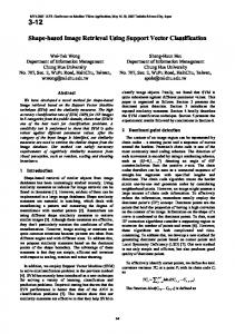
particular semantic descriptions can be approached through some image low-level features. The model of the hierarchical image classification realized in this article is shown in Fig.1. First, we classify the image database into day, night and sunrise/sunset class. To the night and sunrise/sunset image, there is no need to classify it further. So we just classified the day image into close-up and non close-up class. The close-up image includes some enlarge faces, flowers or single objects etc, which will not be classified in this paper further. To the non close-up image, we can classify it into indoor and outdoor class. But to the close-up images, we don’t classified it further. At last we further classified the Image Database
Day
Night
Close-up
Sunrise/Sunset
Non Close-up
1. Introduction Outdoor With the development of science and technology, more and more images are available in the computer from photo collections, web pages, video databases and pictures got by digital camera etc. This has created a great need to develop image management systems that assist the user in storing, indexing, browsing and retrieving images from the vast image database. The present content-based image retrieval (CBIR) system can’t meet the user’s information needs. Users queries are typically based on semantics (e.g., show me a plantation image) and not on image low-level features (e.g., show me a green image) while querying image databases. So if the semantic concepts aren’t identified in the image database, retrieval will not be very efficient and effective. Grouping the image database into semantically meaningful class can greatly enhance the performance of a CBIR system. Our purpose is to show how some
City
Indoor
Landscape
Fig.1. Model of the hierarchical image classification outdoor images into city and landscape image. Fig.2 shows the typical image realized in the image classification, which include day, night, indoor, outdoor, close-up, city, and landscape images. We can infer that the image retrieval accuracy will be improved after this hierarchical classification. For example, if the user wants to find some sunrise image, he/she needn’t to retrieval the image in the whole database, but on the sunrise/sunset class. The retrieval range will decrease half and the accuracy will be improved greatly. A number of attempts have been made to understand the high-level semantics from image using low-level
Page 1
features. Chapelle et al. [3] use SVM to realize histogram-based image classification. They select several classes (include 386 airplanes, 501 birds, 200 boats, 625 buildings, 300 fish, 358 people, 300 vehicle) of the Corel database as the image database, distinguish different kinds of object through the SVM classifier. Szummer et al. [4] use a K-Nearest Neighbor classifier and leave one-out criterion to report classification accuracy, for the indoor vs. outdoor classification problem, of approximately 90% on a database containing 1324 images. They use the color and dominant directions to do the classification. Vailaya et al.[2] propose algorithms for hierarchical image classification. They use VQ based Bayesian Classifier to realize the classification and their system achieved an accuracy of 90.8% for indoor vs. outdoor classification, 95.3% for city vs. landscape classification. The spatial color moment and edge direction histogram were used as the features to classify the indoor vs. outdoor and city vs. landscape image classification respectively. Gorkani and Picard [10] have proposed the use of a multiscale steerable pyramid in 4×4 sub-blocks of 98 images to discriminate between city and suburb scene from photos of landscape scenes. They classify an image as a city scene if a majority of sub-blocks have a dominant vertical orientation or a mix of vertical and horizontal orientations.
the hierarchical image classification were conducted and the results are discussed. Section 5 finally concludes this paper and presents the direction for the future research.
2. Image low-level features used in image classification Table 1. Image features used in the image classification Image Classification Problem
Low-level Feature
Day vs. Night vs.Sunrise/Sunset
CH
Close-up vs. non close-up
CCV and CM
Indoor vs. Outdoor
CM and MRSAR
City vs. Landscape
EDH and TD
We have used several low-level features: color histogram (CH), color moment (CM), color coherence vector (CCV), multi-resolution simultaneous auto-regressive model (MRSAR), edge direction histogram (EDH), Tamura Directionality (TD) to realize the image classification. These features are computed for the whole image and for each sub-block respectively. Table 1 shows the different features used in the image classification. In the following, we will introduce these features respectively.
2.1. Features used in the indoor vs. outdoor classification
Fig.2. (a) night image; (b) sunrise/sunset image; (c) close-up image; (d) and (e) show the typical indoor and outdoor image; (f) and (g) show the typical city and landscape image; The rest of this paper is organized as follows: In section 2, we introduce the image features used for discriminating the different image classes. Training and testing using kernel SVM and its basic theory are discussed in section 3. In section 4, the experiments on
1.Spatial Color Moment Color moment of an image is very simple yet very effective feature for color-based image retrieval [14]. First- and Second-order moments in the LUV color space were used as color features. The image was divided into 4×4 sub-blocks and six features (3 each for mean and standard deviation) were extracted from each sub-block. Indoor images have more uniform illumination and outdoor images, on the other hand, have more varied illumination and chrominance changes. These effects are captured by the spatial color moments, with more variation in the values for typical outdoor images. 2. MRSAR model The MRSAR model constructs the best linear predictor of a pixel based on a non-casual neighborhood [15]. The features used to describe various textures are the weights associated with the predictor. We used three different neighborhoods at scales of 2, 3, and 4 to yield a 15-dimensional feature vector. Each image was divided into 4×4 sub-blocks and MRSAR features were extracted
Page 2
from each sub-block, which is a 240-dimensional feature vector. From the experiment, we concluded that the indoor image yield texture features with low values compared with the outdoor image.
based on whether or not it belongs to a large uniformly-colored region, e.g. a region with area larger than 1% of the image, the CCV classify each histogram bin into two: one represent coherent pixels and the other representing incoherent pixels.
2.2. Features used in the city vs. landscape classification
2.4. Feature normalization
1. Edge direction histogram EDH can be considered as a simple way of characterizing the orientation property. It can be computed by grouping the edge pixels falling into an edge orientation and counting the number of pixels in each direction. A total of 72 bins are used to represent the edge direction histogram; which represent edge directions quantized at 5° intervals. To compensate for different image sizes, we normalize the histograms as follows: H(i) = H(i)/ne, i = [0, …, 71] (1) Where H(i) is the count in bin i of the edge direction histogram, ne is the total number of edge points detected in the image [1] [5]. 2. Tamura directionality The Tamura features are designed based on the psychological studies in human visual perceptions of texture [13]. They correspond to the properties of a texture, which are readily perceived such as coarseness, contrast, and directionality. To compute TD, the gradient vector at each pixel is computed. The magnitude and angle of this vector are defined as ∆G = ( ∆ H + ∆ V ) / 2 (2) θ = tan −1 ( ∆ V / ∆ H ) + π / 2
Where ∆v and ∆H are the horizontal and vertical differences obtained by convoluting the image. Once the gradient have been computed at all pixels, a histogram of θ values, denoted as HD , is constructed by first quantizing θ and counting the pixels with the corresponding magnitude ∆G larger than a threshold. This histogram will exhibit strong peaks for highly directional images and will be relatively flat for images without strong orientation. From the experiment, we can see that the histogram of the city image has stronger peaks than the landscape images. The image was divided into 6×6 sub-blocks and 8 features were extracted from each sub-block (288-dimensional feature vector).
2.3. Features used in the close-up vs. non close-up classification We used spatial CM and CCV as the salient feature to distinguish the close-up and non close-up images, here we just introduce CCV feature. The CCV feature incorporates spatial information into color histogram representation. By classifying each pixel in an image
The image database comes from all kinds of sources, so the image size isn’t consistent. For the sake of computation, all the features were normalized to the same scale as follows: y = ( y − min) /(max − min) (3) Where yi represents the ith feature component of a feature vector y, min and max represent the range of values for the features and y i' is the scaled feature component. '
i
i
3. Learning using support vector machines In this section, we give a brief introduction to SVM. SVM is a learning technique developed by V. Vapnik and his team (AT&T Bell Labs, 1985) [7]. The decision surfaces are found by solving a linearly constrained quadratic programming problem. This optimization problem is challenging because the quadratic form is completely dense and the memory requirements grow with the square of the number of data points. SVM is an approximate implementation of the structural risk minimization (SRM) principle. It creates a classifier with minimized Vapik-Chervonenkis (VC) dimension. SVM minimizes an upper bound on the generalization error rate. The error rate is bounded by the sum of the training-error rate and a term that depends on the VC dimension. SVM can provide a good generalization performance on pattern classification problems without incorporating problem domain knowledge [8].
3.1. Linear support vector machines Consider the problem of separating the set of training vectors belonging to two classes, (x1 , y1), …, (xm , ym), where xi ∈ Rn is a feature vector and yi ∈ {+1,-1} is a class label, e.g., image classification problem, +1 denotes indoor image, -1 denotes the outdoor image. If the two classes are linearly separable, the hyper-plane that does the separation is: ω⋅x + b = 0 (4) The goal of a support vector machine is to find the parameter w0 and b0 for an optimal hyper-plane to maximize the distance between the hyper-plane and the closest data point: y (ω ⋅ x + b) ≥ 1, i = 1,mm (5) For a given w0 and b0 , the distance of a point x from the optimal hyper-plane defined in (5) is: i
i
Page 3
d (ω 0 , b0 , x ) =
ω x+b 0
0
ω
(6)
0
Of all the boundaries determined by w and b, the one that
If we denote α = (α 1 ,�α m ) , the m non-negative Lagrange multipliers associated with constraints (5), our optimization problem amounts to maximizing: 1 L(ω, b, a ) = ω − ∑ α { y [(ω ⋅ x ) + b] − 1} (8) 2 m
2
i
i
i
i =1
Support Vectors
∑
with α ≥ 0 and under constraint
m
i
Hyper-plane
i =1
y α = 0 . This i
i
can be achieved by the use of standard quadratic programming methods. The optimal separating hyperplane has the following expansion: 1 ω = ∑ α y x , b = − ω ⋅ [x + x ] (9) 2 So the hyperplane decision function can thus be written as: f ( x ) = sgn ∑ α y x ⋅ x + b (10) m
0
0
0
i
i
0
r
i
s
i =1
Margin
m
0
i
Fig.3. Illustration of the idea of an optimal hyper-plane for linearly separable patterns and definition of the distance maximizes the margin will generalize better than other possible separating hyper-planes. A canonical hyper-plane has the constraint for parameters w and b: min xi yi [( w ⋅ xi) + b] = 1. A separating hyper-plane in canonical form must satisfy the following constraints,
y
asys
a2y2
K(x2, x)
K(x1, x)
3.2. Kernels of SVM Table 2. Types of kernel functions Kernel Function
K (x, y)
Polynomial
(x ⋅ y + 1) d
Sigmoid K(xs, x)
…
… 1
xn
2
x
x
Fig.4. Illustration of the SVM yi [( w ⋅ xi)
+ b] ≥ 1, i = 1, …m.
The margin is
2 ω
according to its definition. Hence the hyper-plane that optimally separates the data is the one that minimizes 2 1 1 φ (ω) = ω = (ω ⋅ ω) (7) 2 2 2 Since the ω is convex, minimizing it under linear
constraints (5) can be achieved with Lagrange multipliers.
i
Where x r and x s are support vectors which belong to class +1 and –1 respectively. A linear separable example in 2D is illustrated in Fig.3.
Gaussian RBF a1y1
0
i
i =1
exp( −
2 1 x−y ) 2σ 2
tanh(κ ( x ⋅ y ) − µ )
If the two classes are non-linearly separable, the input vectors should be nonlinearly mapped to a high-dimensional feature space by an inner-product kernel k(x, y). Fig.4.shows the basic idea of SVM, which is to map the data into some other dot product space via a nonlinear map and perform linear algorithm in high-dimension space. In which x = ( x 1 , x 2 , � x n ) is the input vector and k ( x i , x) show the inner product with s support vectors. Table 2 shows three typical kernel functions. In our method, we use the Gaussian RBF kernel, because it was empirically observed to perform better than other two. For a given kernel function, the classifier is given by replacing x i ⋅ x with k(x, y).
4. Experiments and discussion Given an input image, the classifier compares the extracted image features with the support vectors and computes the distance and decides which class the image is. For our system, first, the image database is classified
Page 4
as day or night. For the day image, we then classified it as indoor or outdoor or close-up image. If it is outdoor image, we then decide the image is city or landscape. We present classification accuracy on a set of independent test patterns as well as on the training set. The image classifications have been realized based on the single feature and the combination of various features. Through the combination of two SVM classifiers, the accuracy can be improved to some extent. In all the classification experiments, the SVM-light program of Joachims [8] is used in SVM training and classification, and RBF kernel is used.
4.1. Day vs. Night vs. Sunrise/Sunset image classification Table 3. Day vs. night vs. sunrise/sunset classification accuracy (%) Image
Training set Count
Acc.
Day
2200
99.5
Night
580
99.1
Testing set Count
Acc.
3500
95.3
3743
94.9
382
97.5
Sunrise
410 99.0 316 96.2 /Sunset Table 3 shows the classification accuracy for the day vs. night vs. sunrise/sunset classification problem. We conducted the experiment on a database of 11131 images, which includes (962 night images, 9443 day and 726 sunrise/sunset images). We classified the database into 3190 training sets (580 night images, 2200 day and 410 sunrise/sunset image) and the left 7941 testing sets. From this table, we can conclude that CH in HSV space is very effective in this kind of image classification. The SVM is a binary classifier, to solve the threeclasses pattern recognition problem we combine three binary classifiers [11]. We select the “one against the others” to realize the multi-classes problem considering the classification complexity. In this algorithm, 3 hyperplanes are constructed. Each hyperplane separates one class from the other classes. Through comparing the distance from the input data to the three hyperplanes, we can decide which class the input is.
4.2. Close-up vs. Non close-up classification The classification experiments were conducted on the day images (9443), which include 857 close-up image and 8586 non close-up images. We classify the database into 3520 training sets (520 close-up and 3000 non close-up image) and 5923 testing sets. All these images are collected from various sources (Corel stock photo
library, scanned personal photographs, images captured using a digital camera and the Web pages.) and are of varying sizes. Table 4 shows the classification accuracy using CM and CCV features respectively and the combination of the two features. Table 4. Close-up vs. Non close-up classification accuracy (%) Traini Testing set Image ng set Feature class Coun Acc. Acc. t CM 100 92.6 Close-up 337 97.9 CCV 100 93.4 Non close-up
CM CCV
99.8 98.5
90.5 5586
88.9
94.8
4.3. Indoor vs. Outdoor image classification The experiment was conducted on the database of 5187 images, which includes 1443 indoor image and 3744 outdoor image. We select 2878 images as the training set (include 878 indoor and 2000 outdoor images) and the others as the test set. To compare the classification accuracy using different low-level features, the experiment were conducted using CH, CCV, CM, MRSAR texture et al. The best two features for this kind of classification are color moment and MRSAR features. We have fulfilled the indoor vs. outdoor image classification with the combination of the two features, each weight is 0.5. Table 5 shows the classification accuracy, we can conclude that the accuracy is improved than just using one feature. Table 5. Indoor vs. Outdoor Classification Accuracy(%) Traini Testing set Image ng set Feature class Acc. Count Acc. CM 99.8 89.6 Indoor 565 92.8 MRSAR 99.3 88.4 CM 99.5 93.7 Outdoor 1744 95.2 MRSAR 98.9 91.6
4.4. City vs. Landscape image classification The experiment was conducted on the database of 7255 images, which includes 3121 city and 4134 landscape images. The training set is 4305 (2188 city and 2117 landscape) and the test image number is 2950. We conducted this classification using EDH and TD features. The test accuracy using EDH feature can achieve 89.6% and TD 87.5%. Table 6.shows the classification accuracy using the combination of EDH and TD features. The
Page 5
weight of each feature is 0.5. From this table we can conclude that the accuracy has been improved when combining the two features alone. Table 6. City vs. Landscape Classification Accuracy Database
Accuracy
Size
(%)
Training Set
4305
99.6
Test Data
2950
92.8
Entire Database
7255
96.4
Test Data
4.5. Dicussion of experimental results From the classification results, we can conclude that lack of light and the autumn landscape can cause the misclassification of the day image. The presence of the light source or the sunshine through windows or doors seems to be the main cause of misclassification of indoor image. The main reasons for the misclassification of outdoor images are uniform lighting along the image and the dark images. The misclassification of the city images is attributed to the following reasons: (1) long distance city shots; (2) top view of city scenes. Most of the misclassified landscape images have strong vertical edges from tree trunks, the structured bridge, fences, which lead to their assignment to the city class. From the above semantic image classification systems, we can conclude that the image low-level features have limitation in discriminating the image classification problem. So we should add the feedback to this system and improve the man-machine interactive ability. On the other hand, the accuracy of the hierarchical classification depends to some extent on the former classification results. So how to deal with the rejection rate is the main problem in hierarchical classification.
5. Conclusions and future work Image classification is a very challenging task for the image retrieval and management. In this paper, we have presented an approach that uses SVM to realize hierarchical classification of the image database. The experimental results show that this approach is very effective for the image retrieval and management. To the future work, the reject option should be added into the system to improve the classify accuracy. On the other side, how to select small and representative examples as the training set is a difficult problem need to solve for the SVMs. We also need to work on adding an incremental learning paradigm to the classifiers, so that they can improve their performance over time as more training
data is presented. Acknowledgements This work is funded by research grants from the Chinese National 973 Program (Grant No. G1998030502). The first author would like to thank Drs. Hongjiang Zhang, Yongmei Wang and Xiangrong Chen, for the enlightening discussions during her staying at Microsoft Research China. References [1] A. Vailaya, A.K. Jain, and H.J. Zhang, “On Image Classification: City Image vs. Landscapes,” Pattern Recognition, Vol. 31, No. 12, pp.1921-1936, 1998. [2] A. Vailaya, M. Figueiredo, A.K. Jain, and H.J. Zhang, “Content-based hierarchical classification of vacation images”. Proceedings of SPIE - The International Society for Optical Engineering Proceedings of the 1999 7th Conference of the Storage and Retrieval for Image and Video Databases VII Jan 26-29 1999, Vol.3656 San Jose, Ca, USA, pp.415-426, 1999. [3] O. Chapelle, P. Haffner, and V. Vapnik. “SVMs for Histogram-Based Image Classification,” IEEE Trans. on Neural Networks, 10(5): pp.1055-1065, Sep. 1999. [4] M. Szummer and R.W. Picard, “Indoor-Outdoor Image Classification,” IEEE Intl Workshop on Content-based Access of Image and Video Databases, Jan 1998. [5] J. Canny, “A computational approach to edge detection”,IEEE Trans.on Pattern Analysis and Machine Intelligence. 8(6), pp.679-698, 1986. [6] A. Vailaya and A.K. Jain, “Reject Option for VQ-based Bayesian Classification”, Proc. 15the International Conference on Pattern Recognition, September, 2000. [7] V. Vapnik, “The nature of statistical learning theory,” Springer-Verlag, New York, 1995. [8] T. Joachims. “Making large-scale SVM learning practical,” In B. Scholkopf, C. Burges, and A. Smpla, editors, Advances in Kernel Methods-Support Vector Learning. MIT Press, 1999. [9] H-H. Yu and W. Wolf, “Scenic classification methods for image and video databases”, In Proc. SPIE, Digital Image Storage and Archiving Systems, pp.363-371, 1995. [10] M. Gorkani and R.W. Picard, “Texture Orientation for sorting photos at a glance”, In Proc. Int. Conf. Part Rec., Vol. I, pp. 459-464, Oct.1994. [11] J. Weston and C. Watkins. Multi-class support vector machines. Technical Report CSD-TR-98-04, Department of Computer Science, Royal Holloway, University of London, Egham, TW20 0EX, UK, 1998. [12] A. Vailaya, H.J. Zhang, A.K. Jain "Automatic Image Orientation Detection" 1999 IEEE International Conference on Image Processing, Kobe, Japan, Oct. pp.24-28. [13] H. Tamura, S. Mori, and T. Yamawaki, "Texture features corresponding to visual perception," IEEE Trans. System, Man, Cybernet., Vol. 8, No. 6, 1978. [14] M. Stricker and M. Orengo. “Similarity of color images”. In Storage and Retrieval for Image and Video Databases SPIE, Vol. 2420, pp. 381-392, San Jose, CA, February 1995. [15] J.C. Mao and A.K. Jain. “Texture classification and segmentation using multiresolution simultaneous autoregressive models”. Pattern Recognition, pp.173-188, 1992.
Page 6