a comparison of some domain decomposition and ... - Semantic Scholar

A COMPARISON OF SOME DOMAIN DECOMPOSITION AND ILU PRECONDITIONED ITERATIVE METHODS FOR NONSYMMETRIC ELLIPTIC PROBLEMS XIAO-CHUAN CAI

Department of Mathematics, University of Kentucky Lexington, KY 40506, USA

WILLIAM D. GROPP

Mathematics and Computer Science Division Argonne National Laboratory Argonne, IL 60439, USA

DAVID E. KEYES

Department of Mechanical Engineering, Yale University New Haven, CT 06520, USA ABSTRACT In recent years, competitive domain-decomposed preconditioned iterative techniques have been developed for nonsymmetric elliptic problems. In these techniques, a large problem is divided into many smaller problems whose requirements for coordination can be controlled to allow eective solution on parallel machines. A central question is how to choose these small problems and how to arrange the order of their solution. Dierent speci cations of decomposition and solution order lead to a plethora of algorithms possessing complementary advantages and disadvantages. In this report we compare several methods, including the additive Schwarz algorithm, the classical multiplicative Schwarz algorithm, an accelerated multiplicative Schwarz algorithm, the tile algorithm, the CGK algorithm, the CSPD algorithm, and also the popular global ILU-family of preconditioners, on some nonsymmetric or inde nite elliptic model problems discretized by nite dierence methods. The preconditioned problems are solved by the unrestarted GMRES method. A version of the accelerated multiplicative Schwarz method is a consistently good performer. Keywords : domain decomposition, preconditioning, iterative methods, nonsymmetric, inde nite, elliptic problems.

1

1. Introduction The focus of this paper is domain decomposition methods for the solution of large linear systems of nonsymmetric or inde nite elliptic nite dierence equations. In the past ve years, there has been gratifying progress in the development of domain decomposition algorithms for symmetric elliptic problems, and a number of fast methods have been designed for which the condition number of the iteration matrix is uniformly bounded or grows only in proportion to a power of (1+ln(H=h)), where H is the diameter of a typical subdomain and h is the diameter of a typical element into which the subdomains are divided. Such algorithms are often called \optimal" or \nearly optimal" algorithms, respectively, though we note that these adjectives pertain to the convergence rate only, and not to the overall computational complexity. The nearly optimal algorithms may still retain terms that are superlinear in 1=H or in H=h, depending upon how the component problems are solved. For nonsymmetric and inde nite problems, the theory to date is far less satisfactory. Yet, the solution of such problems is an important computational kernel in implicit methods (for instance, Newton-like methods) used in the solution of nonlinear partial dierential equations such as arise in computational uid dynamics. Such a kernel is often CPU-bound or memory-bound or both on the fastest and largest computers available. Furthermore, it may often be the only computationally intensive part of production nite dierence codes whose ecient parallelization is not straightforward, particularly when the distribution of data throughout the computer's memory hierarchy cannot be dictated exclusively by linear algebra considerations. If the parallel solution of nonsymmetric and inde nite problems were truly routine, many applications now solved by various types of operator splitting could be handled fully implicitly. An ecient iterative algorithm for elliptic equations requires a discretization scheme, a basic iterative method, and a preconditioning strategy. There is a signi cant dierence between symmetric and nonsymmetric problems, the latter being considerably harder to deal with both theoretically and algorithmically. The main reasons are the lack of a generally applicable discretization technique for the general nonsymmetric elliptic operator, the lack of \good" algebraic iterative methods (such as CG for symmetric, positive de nite problems), and the incompleteness of the mathematical theory for the performance of the algebraic iterative methods that do exist, such as GMRES [32]. By a \good" method, we mean a method that is provably convergent within memory requirements proportional to a small multiple of the number of degrees of freedom in the system, independent of the operator. One must assume that the symmetric part is positive de nite and be able to aord amounts of memory roughly in proportion to the number 2

of iterations, in order to obtain rapid convergence with GMRES. The task of nding a good preconditioner for nonsymmetric or inde nite problems is more important than for symmetric, positive de nite problems, since, rst, the preconditioner can force the symmetric part of the preconditioned system to be positive de nite, and second, a better-conditioned system implies both more rapid convergence and smaller memory requirements. Domain decomposition methods are commonly classi ed according to a few orthogonal criteria. \Overlapping" and \nonoverlapping" methods are dierentiated by the decomposition into territories on which the elemental subproblems are de ned. Overlapping methods generally permit simple (Dirichlet) updating of the boundary data of the subregions at the expense of extra arithmetic complexity per iteration from the redundantly de ned degrees of freedom. \Additive" (Jacobi-like) or \multiplicative" (GaussSeidel-like) methods are dierentiated by the interdependence of the subregions within each iteration. For the same number of subregions, additive methods are intrinsically more parallelizable. Classi ed according to convergence rate, there are \optimal" algorithms, for which the rate is independent of the number of unknowns as well as the number of subregions; \nearly optimal" algorithms, for which the rate depends on the number of unknowns and subregions through a power of their logarithm at worst; and \nonoptimal" algorithms. Compared in this paper are optimal overlapping algorithms, both additive and multiplicative; a nearly optimal nonoverlapping algorithm, partly additive, partly multiplicative; and a nonoptimal nonoverlapping multiplicative algorithm. Most of the theory concerning the convergence rate of domain decomposition methods is in the framework of the Galerkin nite element method. In some cases the Galerkin results transfer immediately to nite dierence discretizations, though this is less true for nonsymmetric problems than for symmetric. Whereas experimental papers for symmetric problems, such as [20] and [25], predominantly played the role of verifying theory, in this paper we hope to stimulate it. Algorithms based on preconditioned iterative solution of the normal equations are beyond the scope of this paper, though they continue to undergo development [3, 4, 28, 31]. The outline of this paper is as follows. In Section 2, we describe ve domain decomposition methods, their convergence properties, and related implementation issues. Some issues related to parallelism and parallel complexity are discussed in Section 3. Section 4 contains numerical results for four dierent test problems, followed by some brief conclusions in Section 5. An early version of this work has appeared in an abridged proceedings form [8]. This paper completes and supersedes the earlier version. 3

2. Description of Algorithms In this section, we brie y describe all the algorithms under consideration. We give only the formulation used in our experiments but note here that each is representative of a class. For theoretical purposes most of these algorithms are best formulated in terms of the subspace projections de ned by the elliptic bilinear forms. Since we use only nite dierence discretization, matrix notation is more convenient, instead. The convergence rate of each algorithm is given in terms of the spectral bounds of the iteration matrix. These bounds may be related to the number of iterations required by each algorithm to achieve a given accuracy.

2.1. An elliptic problem, a two-level discretization, and notation Let be a two-dimensional polygonal region with boundary @ , and let

(

Lu = f in

u = 0 on @

(2.1)

be a second-order linear elliptic operator with a homogeneous Dirichlet boundary condition. The nite dierence approximation of Dirichlet problem (2.1) is denoted by

Bh uh = (Ah + Nh)uh = fh ; (2.2) where Bh ; Ah and Nh are nn matrices and h characterizes the mesh interval of the grid, which will be referred to as the h-level or ne grid. Here Ah represents the discretization of the symmetric, positive de nite part of the operator L, and Nh represents the remainder. Let (
;
) denote the Euclidean inner product with the corresponding norm k
k. We denote the energy norm associated with the matrix Ah as

k
kA = (Ah
;
) = : The total number of interior nodes of the h-level grid of will be denoted as n. Two nite dierence discretizations are employed alternately for the 1 2

rst-order terms in (2.1), namely, the central and upwinding discretizations. In practice, there are many other discretization techniques such as the arti cial diusion and streamline diusion methods [24] and the methods in [1]. Multiple discretizations can usefully be combined in the same iterative process; see, e.g., [26]. Our methods require a coarse grid over containing n0 interior nodes, or crosspoints, fck ; k = 1;


; n0g; we call this the H -level grid. Bh;0 is an n0  n0 matrix representing the nite dierence discretization of L on the 4

i

i 0

1

2 ?1;2

Fig. 1. The overlapping f i g and nonoverlapping f i g decompositions of

0

H -level grid. Let i; i = 1;


; NS , be nonoverlapping subregions of with diameters of order H , such that  i =  . The vertices of any i not on @

coincide with the h-level nodes. Let ?ij be the intersection of the adjacent pair of subdomains i and j excluding the end points. We refer to the set of subdomains

f i; ?ij ; ck; j 6= i = 1;


; N; k = 1;


; n g 0

as a nonoverlapping decomposition, or substructuring, of ; see Figure 1. When the unknowns are ordered with respect to the substructuring of the region, the stiness matrix Bh can be written in the block form as

1 0 B II BIE BIC Bh = B @ BEI BEE BEC CA ; BCI BCE BCC

(2.3)

where BII is a block diagonal matrix representing the discretization of the independent subregion interior problems, BEE corresponds to the problems on the edges (also called interfaces) excluding crosspoints, and BCC corresponds to the crosspoints. The block matrices with diering subscripts contain the h-scale coupling of the original discretization between points in the dierent sets. Following [10, 15], we can obtain an overlapping decomposition of , denoted by

f i; i = 0;


; N g: 0

5

For i 6= 0, we extend each i to a larger region i which is cut o at the physical boundary of . Let ni be the total number of h-level interior nodes in i , and let Bh;i denote the ni  ni stiness matrix corresponding to the nite dierence discretization of L on the ne grid in i . The size of the matrix Bh;i depends not only on the size of the substructure i but also on the degree of overlap. We reserve the subscript \0 " for the global coarse grid and note that 0 = . Let Ri be an ni  n matrix representing the algebraic restriction of an n-vector on to the ni -vector on i . Thus, if vh is a vector corresponding to the h-level interior nodes in , then Ri vh is a vector corresponding to the h-level interior nodes in i . The transpose (Ri)t is an extension-by-zero matrix, which extends a length ni vector to a length n vector by padding with zero. R0( R0), an n0  n matrix, is somewhat special. It is the neto-coarse grid restriction operator that is needed in any multigrid method. 0

0

0

0

0

0

0

0

0

0

0

0

0

0

0

0

0

2.2. GMRES for the preconditioned system The GMRES method, introduced in [32], is mathematically equivalent to the generalized conjugate residual (GCR) method [17] and can be used to solve the linear system of algebraic equations:

Px = b;

(2.4)

where P is a nonsingular matrix, which may be nonsymmetric or inde nite, and b is a given vector in Rn . The method begins with an initial approximate solution x0 2 Rn and an initial residual r0 = b ? Px0 . At the mth iteration, a correction vector zm is computed in the Krylov subspace

Km(r ) = spanfr ; Pr ;


; P m? r g that minimizes the residual, minz2Km r0 jjb ? P (x + z )jj for some appropriate norm jj
jj . The mth iterate is thus xm = x + zm . According to 0

0

1

0

(

)

0

0

0

the theory of [17], the rate of convergence of the GMRES method can be estimated by the ratio of the minimal eigenvalue of the symmetric part of the operator to the norm of the operator. Those two quantities are de ned by [x; Px] and C = sup jjPxjj ; cP = xinf P 6=0 [x; x] x6=0 jjxjj where [
;
] is an inner product on Rn that induces the norm jj
jj . Following [17], the rate of convergence can be characterized, not necessarily tightly, as follows: If cP > 0, which means that the symmetric part of the operator P 6

is positive de nite with respect to the inner product [
;
], then the GMRES method converges and at the mth iteration, the residual is bounded as m= jjrmjj  (1 ? CcP ) jjr jj; P 2

2

2

0

where rm = b ? Pxm . The algorithm is parameter-free and quite robust. Its main disadvantage is its linear-in-m memory requirement. To t the available memory, one is sometimes forced to use the k-step restarted GMRES method [32]. However, in this case neither an optimal convergence property nor even convergence is guaranteed. Methods generally less rapidly convergent per matrix-vector-multiply than GMRES have recently been devised [19, 34] in order to overcome this limitation. In our applications, we restrict ourselves to preconditioners suciently \strong" that the total number of GMRES iterations is relatively small, and therefore no restarting is required. In the present paper, the linear operator P corresponds to the left- or rightpreconditioned linear system, and b is the properly modi ed right-hand side. The simple L2 inner product, together with its induced norm, is used in Rn .

2.3. Multiplicative Schwarz method (MSM) The multiplicative Schwarz algorithm is a direct extension of the classical Schwarz alternating algorithm, introduced in 1870 by H. A. Schwarz in an existence proof for some elliptic boundary value problems in certain irregular regions. This method has attracted much attention as a convenient computational method for the solution of a large class of elliptic or parabolic equations. The original Schwarz alternating method is a purely sequential algorithm. To obtain parallelism, one needs a good subdomain coloring strategy so that a set of independent subproblems can be introduced within each sequential step and the total number of sequential steps can be minimized. A detailed description of the algorithm and its theoretical aspects can be found in [6, 11, 27]. The coloring is realized as follows. Associated with the decomposition f j g, we de ne an undirected graph in which nodes represent the extended subregions and the edges intersections of the extended subregions. This graph can be colored by using colors 0;


; J , such that no connected nodes have the same color. Obviously, colorings are not unique. Numerical experiments support the expectation that the minimizing the number of colors enhances convergence. An optimal ve-color strategy (J = 4) is shown for the decomposition in Figure 2, in which the total number of subregions (including the coarse grid on the global region) is N + 1 = 17. This algorithm can be employed in the stationary, Richardson sense or as a preconditioner for another algebraic iterative process. Along with the 7 0

? ?

? ?

?

?

?

?

?

? ?

?

?

? ?

?

?

?

? ?

?

?

? ?

?

? ?

?

?

Color 0

Color 1

Color 2

.

Color 3

Color 4

Fig. 2. The coloring pattern of 16 ne grid overlapped subregions and a coarse grid region. Color \0" is for the global coarse grid. The extended subregions of the other colors are indicated by the dotted boundaries.

other algorithms to be described below, we shall normally employ it as a preconditioner for GMRES, but because of its historical importance, and to illustrate certain robustness advantages of acceleration, we also include the Richardson version in our tests. In this paper, we shall use the abbreviation MSM for the multiplicative Schwarz-preconditioned GMRES method, and MSR for the simple Richardson process that corresponds to the classical Schwarz alternating algorithm with an extra coarse grid solver. Letting Bh;0 = Bh;0 and R0 = R0, we describe the MSR algorithm in terms of a subspace correction process. MSR algorithm: Let ukh be the current approximate solution. Then ukh+1 is computed as follows. For j = 0; 1;


; J : (i) Compute the residual in subregions with the j th color: 0

0

j

j

rhk+ J+1 = fh ? Bhuhk+ J+1 :

(ii) Solve for the subspace correction in all i s that share the j th color: 0

j

j

Bh;iehk+ J+1 = Rirhk+ J+1 : 0

0

(iii) Update the approximate solution in all i s that share the j th color: 0

j

j+1

j

uhk+ J+1 = uhk+ J+1 + (Ri)t ehk+ J+1 : 0

At each iteration, every subproblem is solved once. For j 6= 0, applications of operators Rj and (Rj )t do not involve any arithmetic operations. 8 0

0

For j 6= 0, within each series of steps (i){(iii), the operations in subregions sharing the same color can be done in parallel. Let us de ne the n  n matrices

Mi?1 = (Ri)t(Bh;i )?1 Ri and Pi = Mi?1 Bh ; for i = 0;


; N: 0

0

0

For j = 0; 1;


; J , if we denote Qj as the sum of all Pi s and Nj?1 as the sum of all Mi?1 s that correspond to subregions of the j th color, then MSR can be written in the following more compact form: For a given initial approximate solution u0h , and k = 0; 1;


, 0

0

ukh+1 = ukh + (I ? EJ +1 )(fh ? Bh ukh ) = EJ +1 ukh + fh ; where the error propagation operator EJ +1 is de ned as EJ +1 = (I ? QJ )


(I ? Q0 ) and fh  ghJ is computed at a pre-iteration step by the following J + 1 0

0

sequential steps:

gh0 = N0?1fh gh1 = gh0 + N1?1 (fh ? Bh gh0 ) .. .

ghJ = ghJ ?1 + NJ?1 (fh ? Bh ghJ ?1 ):

Next, we shall discuss an accelerated version of MSR. We begin with the observation that if the matrix I ? EJ +1 is invertible, then the exact solution of equation (2.2) also satis es (I ? EJ +1 )uh = fh ; (2.5) 0

which is sometimes referred as the transformed, or preconditioned, system corresponding to (2.2). We next observe that for a given vector vh 2 Rn , the matrix-vector product (I ? EJ +1 )vh , denoted as vhJ , can be computed in a manner similar to that of fh , namely, 0

vh0 = Q0 vh vh1 = vh0 + Q1 (vh ? vh0 ) .. .

(2.6)

vhJ = vhJ ?1 + QJ (vh ? vhJ ?1 ): Now, the multiplicative Schwarz preconditioned GMRES method (MSM) can be described as follows: Find the solution of equation (2.2) by solving 9

the equation (2.5) with the GMRES method for a given initial guess and inner product. Even in the case that the matrix Bh is symmetric positive de nite, the iteration matrix I ? EJ +1 is not symmetric. An obvious symmetrization exists, upon which a conjugate gradient method can be used as the acceleration method; however, we shall not emphasize the case of a symmetric Bh in this paper. Inexact subdomain solves can easily be incorporated with either MSR or MSM. For i 6= 0, let B~h;i be an ni  ni matrix that is spectrally equivalent to Bh;i . Then MSR or MSM with an inexact solver can be prescribed as follows: Repeat the preceding derivation except for the replacement of (ii) with 0

0

0

0

j

j

B~h;iekh+ J+1 = Rirhk+ J+1 : 0

0

Many inexact variants of the methods can be formulated. For example, for j 6= 0, let Ah;j denote the matrix corresponding to the central dierence discretization of the Poisson operator in the subregion j . Then step (ii) can be carried out by 0

0

j

j

Ah;j ehk+ J+1 = Rj rhk+ J+1 : 0

0

Note that a \fast" solver, such as one based on FFTs, can now be applied. Using an inexact solver for the interior subproblems, or an exact solver for approximate interior subproblems, can signi cantly reduce the overall computational complexity. This is, in fact, one of the major advantages of domain decomposition methods, in that they allow the use of fast solvers designed for special dierential operators on regions of special shape. A somewhat disappointing experimental observation is that inexact solutions seem not to work well for the coarse grid solver. In fact, the existing theory for MSM [11], as well as the theory for ASM [10], requires an exact solve on the coarse grid. In the piecewise linear nite element case, the convergence of MSR has been proved in [11], under certain assumptions. The rate of convergence is

kukh ? uhkA 

s

1 ? (JC+MSR1)2

!k

kuh ? uhkA; 0

where CMSR > 0 is a constant independent of h, H and J . The estimate holds in both two- and three-dimensional spaces. The assumptions include: (1) the overlap is uniform and must be O(H ); (2) H must be suciently small; and (3) the number of colors, J , must be independent of the size of 10

the subregions H . The same estimate, with a dierent constant, holds for MSR with either exact or spectrally equivalent inexact solvers. For the accelerated version MSM, under the same assumptions, we have that there exist two constants CMSM > 0 and cMSM > 0, independent of both h and H , such that the transformed system is uniformly bounded:

k(I ? EJ )xkA  CMSMkxkA; 8x 2 Rn; +1

(2.7)

and the symmetric part of the transformed system is positive de nite in the inner product (Ah
;
): (Ah (I ? EJ +1 )x; x)  cMSM kxk2A ; 8x 2 Rn :

(2.8)

2.4. Additive Schwarz algorithm (ASM) An additive variant of the Schwarz alternating method was originally proposed in [13, 14, 30] for selfadjoint elliptic problems and extended to nonselfadjoint elliptic cases in [7, 10]. The idea is simply to give up the data dependency between the subproblems de ned on subregions with dierent colors, as in going from Gauss-Seidel to Jacobi. Instead of iterating with (2.6), one uses

vh0 = Q0 vh vh1 = vh0 + Q1 vh

(2.9)

.. .

vhJ = vhJ ?1 + QJ vh : Of course, similar changes have to be made to the right-hand side vector. Coloring does not play a role at all in (2.9). Because of the lack of data dependency, the method is usually not to be recommended as a simple Richardson process, but as a preconditioner for some algebraic iterative methods of CG type. We denote by MASM the preconditioning part of (2.9). Following [10] and using the notation of the previous subsection, we can de ne the inverse of the matrix MASM , referred to as the additive Schwarz preconditioner, as ?1 = (R0)t(Bh;0 )?1 R0 + (R )t(B )?1 R +


MASM 1 1 h;1 +(RN )t(Bh;N )?1 RN : 0

0

0

0

0

0

(2.10)

The key ingredients for the success of the ASM are the use of overlapping subregions and the incorporation of a coarse grid solver. At each iteration, all subproblems are solved once. It is obvious that all subproblems are independent of each other and can therefore be solved in parallel. 11

To obtain an optimal convergence rate, one does not have to solve these subproblems exactly. As proposed in [10], the following preconditioner is also optimal: ?1 = (R0)t(Bh;0 )?1 R0 + (R )t(B~ )?1 R +


M~ ASM 1 1 h;1 (2.11) +(RN )t(B~h;N )?1 RN : 0

0

0

0

0

0

The B~h;i are those de ned in the previous subsection. It has been shown [7, 10] that, in the piecewise linear nite element case, both preconditioners ?1 and M ?1 are optimal under the same rst two assumptions made for ~ ASM MASM MSM in the sense that there exist two constants CASM > 0 and cASM > 0, which may be dierent for exact and inexact subdomain solvers and are independent of both h and H , such that the preconditioned linear system is uniformly bounded: 0

? Bh xkA  CASM kxkA ; 8x 2 Rn kMASM 1

(2.12)

and the symmetric part of the preconditioned linear system is positive de nite in the inner product (Ah
;
) ?1 Bh x; x)  cASM kxk2 ; 8x 2 Rn : (Ah MASM A

(2.13)

In the case Bh = Ah , which means that the original elliptic operator is symmetric positive de nite, the left-preconditioned system is symmetric positive de nite in the (Ah
;
) inner product; thus one can use a CG method. In the nonsymmetric case, the preconditioned system is nonsymmetric regardless of inner product. Therefore, instead of the Ah -inner product, we use the Euclidean inner product for the implementation presented in this paper. By giving up the symmetry requirement of the preconditioned system, we could also use ASM as a right-preconditioner. Neither of the pair of estimates (2.12) and (2.13) has been proved in the L2 norm, but in the numerical experiments section, variability in ASM convergence rates measured (as is customary) with respect to L2 residuals clearly diminishes as mesh and subdomain parameters are both re ned, leading us to conjecture that analogous results hold. The ASM discussed in this subsection can be used recursively for the solving the subdomain problems. The result is the multilevel ASM, as developed in [2, 16, 39].

2.5. Coarse grid plus SPD preconditioning (CSPD) The low-frequency modes of the error are the hardest to damp with nearly any iterative method. Therefore, a direct solver is usually employed on the 12

coarse grid, as in multigrid methods. In the case of nonsymmetric problems, it is even more important to employ a direct coarse grid solver. Based on this observation, it is proved in [38] that a good preconditioner for Bh can be constructed by combining a properly weighted coarse-grid matrix, obtained by discretizing the original nonsymmetric elliptic operator, and some local symmetric positive de nite matrices, obtained by discretizing the symmetric positive de nite part of the elliptic operator. Other methods making special use of the coarse-grid matrix can also be found in [3, 37]. For a symmetric, positive de nite elliptic problem, many good preconditioners are available. Supplemented by an additional coarse-mesh preconditioner, they may become good, sometimes optimal, preconditioners for nonsymmetric problems, as shown in [38]. More precisely, let A~h be a spectrally equivalent symmetric, positive de nite preconditioner for Ah , which is in turn the symmetric, positive de nite part of Bh . Then the new preconditioner can be written as ?1 = ! (R0)t(Bh;0 )?1 R0 + (A~h )?1 ; MCSPD (2.14) where ! > 0 is a balancing parameter. In this paper, the symmetric, positive de nite preconditioner (A~h )?1 is taken as the symmetric, positive de nite additive Schwarz preconditioner. For i = 0;


; N , we denote by Ah;i an ni  ni matrix that corresponds to the discretization of the second-order terms of L in i with homogeneous boundary conditions. Then, we have (A~h )?1 = (R0)t (Ah;0)?1 R0 + (R1)t (Ah;1)?1 R1 +


(2.15) +(RN )t(Ah;N )?1RN : To obtain the optimal ! , one needs to know, in some sense, how good the preconditioner (A~h )?1 is. In our numerical experiments, which use (2.15) in (2.14), the choice of ! = 1:0 is acceptable. The issue of nding the optimal ! in the general case is not fully understood, but seems not to be critical. The coarse-grid-plus-SPD-preconditioner (CSPD) method was analyzed in [38]. Suppose that the minimal and maximal eigenvalues of the preconditioned symmetric, positive de nite part (A~h )?1 Ah are 0 and 1. Then, if the coarse-mesh size, H , is ne enough, there exists a constant ! , depend?1 is an optimal preconditioner for Bh in ing on 0 and 1, such that MCSPD the (Ah
;
) inner product. That is, there exist constants CCSPD > 0 and cCSPD > 0 such that ?1 Bh xkA  CCSPDkxkA ; 8x 2 Rn kMCSPD (2.16) and ?1 Bh x; x)  cCSPDkxk2 ; 8x 2 Rn : (Ah MCSPD (2.17) A 13 0

0

0

0

0

0

0

0

0

0

It is clear that if (A~h )?1 is an optimal preconditioner for Ah , which means that both 0 and 1 are independent of h and H , then with such an ! , also independent of 0 and 1 , the convergence rate of the preconditioned nonsymmetric system is independent of h and H . Although the analysis given in [38] holds only in the Ah inner product, and it is not known whether results similar to (2.16) and (2.17) hold in the Euclidean inner product, we again mention that all error and residual measurements behind Table 7 and Figure 7 are in L2.

2.6. Tile algorithms (GK90/GK91) The tile algorithm, proposed in [22], is designed especially for two-dimensional nonsymmetric problems and can be characterized as a nonoverlapping, multiplicative method. Numerical experiments indicate that the method converges at a rate that deteriorates logarithmically in the ne-mesh parameter, with the coarse-mesh size xed. This method has been tested for a large class of linear and nonlinear problems on various parallel machines [23]. Our tables include results labeled GK90 and GK91. The GK90 preconditioner is

1? 0 0 I B II BIE BIC C B B ? I TEE BEC A @ MGK = @ 1

1

Bh;0

WE WC

1 CA ;

(2.18)

where the matrix TEE is the so-called tangential interface preconditioner, a block diagonal matrix in which each block corresponds to the interface between a pair of neighboring subdomains. The coecients of each block can be obtained by the usual three-point discretization of the \tangential part" of the underlying dierential operator, that is, the set of terms that remain when the operator is expressed in terms of local tangential and normal derivatives and all normal derivatives are then dropped. The matrices WE and WC de ne a so-called ramp-weighted averaging method used to modify the right-hand side of the coarse mesh problem involving Bh;0 . WC is diagonal with all positive elements, all elements of WE are nonnegative, and their rows together sum to unity. A detailed description can be found in [22]. To perform the triangular solve, one needs three sequential steps: solution of a coarse mesh problem with a locally averaged right-hand side; solution of the interface problems with right-hand sides updated by the boundary values provided by the coarse grid solution; and solution of the interior problems with right-hand sides updated by the boundary values provided by the coarse grid and interface solutions. Note that the second and third 14

steps are composed of completely independent subtasks on each interface and subdomain. ?1 It is observed in [22] that some additional saving can be achieved if MGK is used as a right-preconditioner, because then a simple calculation shows that 10 0 1 I I 0 0 CA ; ?1 = B I Bh MGK @    CA B@

  

WE WC

where  denotes a nonzero block. The identity block row means that O(h?2 ) of the unknowns in the Krylov vectors can go untouched (except for scaling) throughout the entire solution process until the preconditioning is unwound in the nal step, after the interface and crosspoint values have converged. Since BII?1 is needed to advance the solution on these separator sets, we cannot escape solving subdomain problems, but substantial arithmetic work is saved. A more recent tile algorithm (GK91) incorporates an additional re nement. The right-hand side of each interface problem is modi ed prior to its solution using TEE to include an approximation to the nontangential terms of the PDE on the interface. These terms are formed from bivariate interpolation of the coarse-mesh solution, quadratic normal to the interface and linear tangential to it. As is apparent from the tables to follow, the additional sequential stage can have a substantial impact on the convergence rate of the tile algorithm without any additional subdomain solves per iteration. The extra communication required, relative to GK90, is all of near-neighbor type. The GK91 preconditioner, written out in factored form, is

0 BII ? =B I MGK @

10 1? 0 I B B IE IC CA B@ I TEE CA B I @

1

I

I

10 0 I B@ I [BEC ? NEC ] CA B@ I I

1? 0 CA B@ I I 1

1? CA

1

1

I

1 CA :

WE WC Bh;0 The normal derivative corrections are in the NEC term. The three sequential I

solves shown are optionally followed by a relaxation step for the crosspoints on the ne-grid. 15

2.7. Substructuring algorithm (CGK) The CGK algorithm, developed in [9], was motivated by the tile algorithm of [22] and also the iterative substructuring algorithm of [5]. Its major dierences relative to the tile algorithms are that it needs an extra set of interior solves and that the interface and interior solves are made independent of the coarse-grid problem. The rst allows a proof of near-optimal convergence rate, and the second oers more exible parallelization. When solving a highly nonsymmetric problem, one must use a coarse grid that is often too large to be handled by a single processor or solved redundantly in each processor. The independence of the coarse-grid problems from the others makes it possible to solve the coarse-grid problem on a collection of MIMD processors, while other processors perform interface and interior problems in parallel. The major dierence between CGK and the BPS-I algorithm [5] for SPD systems is that the coarse-grid solve depends sequentially on the interface and interior solves in BPS-I. The price for the extra parallelism in CGK is that the convergence bound suers an extra factor of (1 + ln(H=h)), as seen below. The nearly optimal, nonoverlapping, partly additive, partly multiplicative CGK method can be expressed as ?1 = (R0)tB ?1 R0+ MCGK h;0

0 ? ? BEI B ? ?B ? BIE K ? 0 1 (2.19) + BII? BIE KEE B EE II II B@ ?K ? BEI B? ?II KEE 0C A; EE II 1

1

1

1

1

1

1

1

1

0

0

0

where KEE is a block diagonal matrix, and each block corresponds to an interface. In our current implementation, every block in KEE has the form of the square root of the negative one-dimensional Laplacian along the interface, with size equal to the number of interior interface nodes. There are other possibilities for KEE (see, e.g., [12]) which better adapt the preconditioner to nonsymmetric and variable coecient problems. ?1 uh , one needs to solve a coarse-grid problem To form the action of MCGK and, at the same time, solve sequentially three sets of subproblems: a rst set of independent interior problems, a set of independent interface problems, and another set of interior problems. This algorithm is analyzed in [9] for a piecewise linear nite element discretization in R2 . The convergence rate degenerates logarithmically with the grid size. More precisely speaking, there exists a small positive constant 16

Table 1 The sequential stages of the algorithms as well as BPS(I)

MSR MSM ASM CSPD GK CGK BPS(I) 1 1 3 3 4

J +1 J +1 H0, such that if

H (1 + ln(H=h)3)  H0 holds, then one has ? Bh xkA  CCGKkxkA ; 8x 2 Rn kMCGK 1

(2.20)

and ?1 Bh x; x)  cCGK =(1 + ln(H=h)3)kxk2 ; 8x 2 Rn ; (Ah MCGK A

(2.21)

where CCGK and cCGK are positive constants independent of H and h but possibly dependent on H0 . It was also proved that if the matrix Bh is symmetric positive de nite, then the estimates are independent of H0 ; in other words, the coarse grid does not need to be \suciently small" in this case.

3. Parallelism and Complexity Analysis In this section, we discuss some the issues of parallelism and parallel arithmetic complexity of the algorithms described in the preceding section. A natural measure of the parallelism of an algorithm is the number of sequential stages it contains. Normally, parallelization can be accomplished only within each stage and not between the stages, which act as synchronization points. The counts of sequential stages for the six preconditioner algorithms introduced in the preceding section, as well as for the BPS(I) algorithm of [5], are summarized in the Table 1. For convenience in providing a simpli ed parallel complexity analysis, focusing only on computer architecture-independent factors, we begin with the assumption that each subdomain is undivided in the mapping onto processors. Furthermore, we assume that all interior problems, de ned on any unextended substructures, are of relatively the same size and require tI unit time (or number of arithmetic operations) to solve. Of course, tI depends not only on how many unknowns each subregion has but also on the method 17

used to solve the interior problem. Similarly, we denote by tI the time required for the interior problems on extended subregions, tC for the crosspoint problem, tE for each interface problem. Let ovlp denote the overlapping factor, which is de ned as the ratio of the number of protruding h-level grid points in i relative to the number of h-level grid points on a side of i. If we assume that the complexity of the subdomain solve is proportional to leading order to the th power of the number of gridpoints, then, approximately, 0

0

tI = (1 + 2ovlp ) d
tI ; 0

Here, d (= 2 or 3) is the dimension of the problem, and a uniform overlap is assumed in all directions. We are able to recommend a small ovlp in practice, corresponding to just one or two ne mesh cells, but we include examples below that use 50% overlap, implying that every point not on a separator belongs to at least two dierent interiors. The interface arithmetic complexity tE can usually be ignored compared with tI or tC , at least for two-dimensional problems. The times tI and tC depend heavily on what kind of solver being used. For example, if each interior dierential operator is approximated by a constant times the Laplacian, a uniform grid is used on the square subregion, and the matrix is suitably preprocessed, then the work of the FFT-based fast Poisson solver is approximately

tI = O((n=N ) log2 (n=N )); where the term n=N corresponds approximately the number of h-level grid points in i . Sometimes a multiple of the Laplacian is not good enough to approximate the interior matrix, and then the original matrix may be used. In this case, a more expensive banded direct solver is used and

tI = O((n=N )(2?1=d)): Other, more ecient solvers for the interior problems have been developed. For example, a few cycles of multigrid or a few Gauss-Seidel iterations perform well for some test problems, as in [2] or [33]. The crosspoint matrix is usually obtained by discretizing the original dierential equation. Using an approximate operator in this case usually results in large iteration counts for our nonsymmetric problems, for reasons that are not yet explained theoretically. A banded direct solver for the crosspoint system needs approximately

tC = O(N (2?1=d)): 18

For i 6= 0, the actions of the restriction and extension operators Ri , Ri, (Ri)t , and (Ri ) on vectors do not involve any arithmetic operations. This is not the case for the coarse-grid problem. If one uses the piecewise linear interpolation, based on the coarse-mesh triangulation shown for \Color 0" in Figure 2, then the cost of applying R0 and (R0)t is approximately 6n. Other restriction and extension operators, such as those usually used in multigrid methods, may also be applied. We denote by t0 the number of arithmetic operations for applying the coarse grid interpolation operator. In the tile algorithms a ramp-weighted averaging method is used to calculate the right-hand-side of the coarse-mesh problem at each GMRES iteration. This method uses p the ne-mesh values only on the interfaces. Approximately t0;GK  4N n=N ops are needed. In GK91 an comparable additional number of ops are needed to adjust the right-hand sides of the interfacial systems with the non-tangential corrections. Neither form of the tile algorithm requires an O(n) interpolation from the crosspoint to the subdomain interior degrees of freedom, or back again. The complexity of the GMRES method was analyzed in [32]. Since we consider only the ve-point nite dierence discretization, the action of the stiness matrix on a given vector requires approximately 5n ops. In the sequential case, I steps of GMRES require I (I +2)n + I (5n) multiplications. For simplicity, we identify the number of ops with the number of multiplications. The parallel arithmetic complexity of GMRES, with p processors, is then approximately   C (I; p) = I (I + 1) n + log (p) + I n + I 5n ; 0

0

GMRES

p

2

p

p

where the term I (I + 1)( np + log2 (p)) is from the dot products and DAXPYs of the Gram-Schmidt process, the term np I from the forming of the new approximate solution after I steps are complete, and 5pn I from the matrixvector multiply. The parallel arithmetic complexity is estimated in Table 2 for p equal to the number of subproblems and in Table 3 for p less than the number of subproblems. It is also important to consider the parallel communication complexity, though its impact is architecture dependent. Whether the sequential stages of Table 1 are enforced by barriers or by the arrival of data, they contribute a term proportional to the message latency of the multiprocessor. The global inner products and matrix-vector products of GMRES p also add latency terms. In addition, an amount of data proportional to n=N and the discrete width of the overlap must be communicated in both directions over each boundary at least once in each preconditioner application. Finally, 19

Table 2 The parallel complexity of the algorithms with the number of processors p equal to the number of subproblems

Method Number of iterations I= MSR O(1) MSM O(1) ASM O(1) CSPD O(1) GK CGK O(1 + ln(H=h))3

Total ops p = number of subproblems  I JtI + tC + tp0 + 5 np   CGMRES (I; p) + I JtI + tC + tp0   CGMRES (I; p) + I maxftI ; tC g + tp0 same as ASM   t CGMRES (I; p) + I tI + tC + tE + 0 pGK   CGMRES (I; p) + I maxf2tI + tE ; tC g + tp0 0

0

0

;

Table 3 The parallel complexity of the algorithms with the number of processors p less than the number of subproblems

Method Total ops p  number of subproblems  MSR I J (N=Jp ) t + tC + tp0 0

I

 

0

MSM

CGMRES (I; p) + I J (N=Jp ) tI

ASM CSPD GK CGK

CGMRES (I; p) + I

 

+ tC + tp0

maxf Ntp ; tC g + tp0 0

I

same as ASM   t0 GK + CGMRES (I; p) + I Ntp + tC + 2Nt p p   t0 CGMRES (I; p) + I maxf2 Ntp + 2Nt ; t g C + p p ;

E

I

I

E

the global coarse grid problem constitutes (either in its setting up or in its solution) a communication bottleneck. For an extended discussion of the parallel communication complexity of domain decomposition algorithms for two-dimensional problems, see [21].

4. Numerical Experiments In this section, we present some numerical results obtained by applying the aforementioned algorithms to

(

Lu = f in

u = 0 on @ ; 20

(4.1)

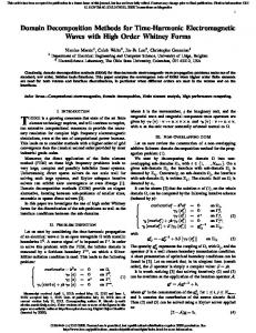
where dierent elliptic operators L will be speci ed and = [0; 1]  [0; 1]. In all cases, the exact solution u = exy sin(x) sin(y ), and f can thus be set accordingly. The unit square is subdivided into two-level uniform meshes, with h and H representing the ne- and coarse-mesh sizes. The elliptic operator is then discretized by the usual ve-point central or upwind dierence methods over both meshes. The full GMRES method, without restarting, is used for all of the left-preconditioned linear systems (except for MSR) in the usual Euclidean norm with zero initial guess. The stopping criterion is the reduction of the initial (preconditioned) residual by ve orders of magnitude in the L2 norm, namely (rk ; rk )1=2  10?5 (r0; r0)1=2; where rk = M ?1 (fh ?Bh ukh ), for k  0, and M ?1 is one of the preconditioners discussed previously. We remark that this stopping criterion is preconditioner dependent. Let ek = u ? ukh be the true error. The preconditioned residual rk = M ?1 Bh ek re ects the true error only if the preconditioner is so strong that both

k(M ? Bh )? kL2 and kM ? Bh kL2 1

1

1

are close to order one. From the nite element theory associated with most of the methods, this is true asymptotically in H and h if the L2 norm is replaced by the energy norm k
kA . To see whether this is so in the range of mesh, subdomain, and problem parameters in our experiments, we take advantage of the exact solution to complement the residual-based iteration count data of Tables 4 through 7, with plots of the true error as a function of iteration index in Figures 3 through 7. We point out some cases in which monitoring the residual does not give a complete picture of the relative quality of dierent methods. Unfortunately, this is probably often the case for results reported in the literature for nonsymmetric elliptic problems; however, in many situations authors have no other practical recourse than to base convergence on (preconditioned) residual. Incomplete LU (ILU) decomposition [29] results are shown for zero, one, and two levels of ll [35]. Double precision is used throughout. Only machine-independent information, namely, the iteration count and true error as a function of iteration, is presented. Throughout this section, we use \ovlp" to denote the size of overlap. That is to say, the distance between the boundaries of an extended subregion and the original subregion p is equal to \ovlp" except near corners, where it can be up to a factor of 2 greater. 21

10 1

+ x *o

10 0

x

x

x x

o *o + x x + *

true error

10 -1

x + *o

10 -2

x o * + x x + xo * + *o

x xo + * x + x * o +

10 -3

x

*o

x + x *o

x

x + x *o

+ x + * +

x

10 -5

*o

x + *o +

0

2

4

x x + *o +

* + o *o

6

x

x

o

10 -4

x

x + *o

x *o +

x x x +

x x x +

o * + x *o + *

8

x x

x

x

x

x x x

o * x + o * + *

10

+ x *o + *o + *

+ x + * + *o

12

x x + x + *o

+ x + *o *

14

x x + + *o *

16

iteration count

Fig. 3. The L norm true error reduction of the Poisson equation with h = 1=128 and = 1=4. \solid x": MSR(ovlp=h); \solid +": MSR(ovlp=2h); \solid  ": MSR(ovlp=4h); \solid o ": MSR(ovlp=8h); \dashed x": MSM(ovlp=h); \dashed +": MSM (ovlp=2h); \dashed  ": MSM(ovlp=4h); \dashed o ": MSM(ovlp=8h); \dotted x": ASM(ovlp=h); \dotted +": ASM(ovlp=2h); \dotted  ": ASM(ovlp=4h); \dotted o ": ASM(ovlp=8h); \dashdot": CGK; \dashdot x": GK91. 1

H

4.1. The Poisson equation Our rst test problem is the Poisson equation

Lu = ? 4 u: Although this is a symmetric problem, we still use GMRES as the outer iterative method. For symmetric positive de nite problems, the iteration matrices of ASM and CGK are symmetric positive de nite; therefore, with a suitable inner product, CG is more ecient. The iteration matrices of MSM, MSR, and the tile algorithm are nonsymmetric. CSPD is not designed for such a test problem and therefore is not tested. The iteration counts are given in Table 4. (Entries that would have required overlap greater than 50% are left blank.) Among all algorithms with small overlap, the MSM takes the least number of iterations. Since MSR does not depend on an outer algebraic iterative method such as GMRES, it requires the least amount of computer memory. Within each group of columns sharing a common H , the iteration counts are constant along diagonals of the table for the overlapping methods (MSR, 22

Table 4 Iteration counts for solving the Poisson equation. The overlapping factors for MSR are given as the subscript of iteration numbers. The corresponding overlapping factors for MSM and ASM are the same as that for MSR and are therefore omitted. The number, such as (2h), which appears next to the name of each method indicates the size of overlap. h?1 =

32

Methods MSR(h) 7( 18 ) MSR(2h) 6( 14 ) MSR(4h) 5( 12 ) MSR(8h) MSM(h) 5 MSM(2h) 5 MSM(4h) 4 MSM(8h) ASM(h) 11 ASM(2h) 11 ASM(4h) 10 ASM(8h) GK91 14 CGK 12

64 128 32 H = 1=4 11( 161 ) 19( 321 ) 6( 14 ) 7( 81 ) 11( 161 ) 5( 12 ) 6( 41 ) 7( 81 ) 5( 12 ) 6( 41 ) 6 7 4 5 6 4 5 5 4 5 13 15 10 11 13 10 11 11 10 11 19 28 9 13 13 12

64 128 64 128 H = 1=8 H = 1=16 7( 18 ) 10( 161 ) 5( 14 ) 6( 18 ) 6( 14 ) 7( 81 ) 4( 12 ) 5( 14 ) 5( 21 ) 6( 41 ) 4( 12 ) 1 5( 2 ) 4 5 3 3 4 4 3 3 4 4 3 4 10 11 9 8 10 10 8 8 10 10 8 10 17 32 9 16 11 11 10 10

MSM and ASM). The ratio ovlp H is the same for each case along a diagonal, as tabulated in parentheses. This suggests that the iteration count depends only on the ratio ovlp H , but not on the actual mesh sizes h or H . This observation has recently been proved in [36]. The true error reduction curves corresponding to some entries of the H = 1=4, h = 128 column of Table 4 are given in Figure 3. The multiplicative Schwarz preconditioned GMRES with suciently large overlap takes the least number of iterations to reduce the initial error to the discretization error. We also note that the curve for the nonoverlapping method CGK is very close to the curve for ASM with the minimum amount of overlap.

4.2. A nonsymmetric problem Our second test problem is a nonsymmetric, constant coecient problem corresponding to a uniform convection skewed at 45 to the coordinate axes: Lu = ? 4 u + ux + uy : We specify dierent values for the constant convection strength  > 0 in Table 5. The rst-order terms of the elliptic operator are discretized by two 23

10 1

+ x *o

10 0

x + * o + x

x + *

x + *

* o

* o

+ x

10 -1

x + *

* o

+ x

x + *

o *

true error

x +

x +

o

o *

x

x + *

x + *

x +

o *

*o

x

+

x +

*

x

* o

* o

*

o

*o +

x

x + *o

10

x + *o

x + *o

x

x

x

x

x

+ +

* *

+

*

+

* *

o

* * * *

o o

x

o

x x + x *o

x

+

o

+ x *o

x

+

x

+ x + *o

x

* *

x

x + *o

x

+

o

+ x + *o

x

+

o

+ x

*

o

+ x * +

x

+

*

x

+ x *

x +

*

x

*

5

x + *

+

o

0

o *

x

o

x + *

*

+

+

10 -3

x + *

x +

+ x *

x + *

o *

x + o *

10 -2

x + *

* *o

x + * x + o

10 -4

x + *

+ x *o

15

x + x *o

x x + *o

x x + *o

20

xo x + *

xo x + *

o xo x + *

+ * * o xo x + *

*

+

* *o x x + *o

25

* o x x + *o

xo x + *o

* xo x + *

+ * x x + *o

+ x *o x + *

30

iteration count

Fig. 4. The L norm true error reduction of the central dierenced nonsymmetric problem with parameters  = 50, h = 1=128 and H = 1=8. \solid x": MSR(ovlp=h); \solid +": MSR(ovlp=4h); \solid ": MSM(ovlp=h); \solid o": MSM(ovlp=4h); \dotted x": ASM(ovlp=h); \dotted +": ASM(ovlp=4h); \dotted ": CSPD(! = 1:0); \dotted o": CGK; \dashed": GK91; \dashdot x": ilu(0); \dashdot +": ilu(1); \dashdot ": ilu(2). 1

schemes, namely, the central dierence method for  of O(h?1 ) or less and the upwind-dierence method for larger  . When using the central dierence method, for a xed ne mesh size h?1 = 128, we observe that as  is increased beyond a certain size (near 10), all methods, except MSM with sucient overlap, show a sharp upturn in the iteration count. The MSR loses convergence if  is larger than this transitional  for essentially all overlapping sizes. All other GMRES-based methods continue to converge but at a slower rate, especially the nonoverlapping methods. The nonoverlapping methods with uncorrected interfaces have diculty handling large convection terms; however, GK91 improves in this limit and even surpasses ASM when H ?1 = 4. Even when GK91 trails ASM in iteration count based on a xed preconditioned residual reduction, its true error versus iteration count curve lies mostly below that of ASM. Distinct from all other methods, MSM converges in a small number of steps that, in cases of generous overlap, is almost independent of the strength of convection. The error reduction curves that correspond to the column h = 1=8,  = 50 in the upper half of Table 5 are given in Figure 4. The general complexion changes when we switch to the upwind-dierence method. The iteration counts for the overlapping methods remain nearly 24

10 1

+ x *o

10 0

x *o x + * *o x +

x * + + * x

true error

o x + * o

10 -1

10 -2

0

* x + * + x

* x + + x *

* x

x *

x *

x *

* x

* x

x

x o

*

*

+ *

+

+

o

*o

*o

x *o +

5

* x

+

x o

* x

x + + *o + *o x

*

*

x x + xo + + *o

*

*

* *

x

x o + + x *o

*

x + o + x *o

10

+ x *o

x + *o

x + *o

+ x *o

+ x *o

* x + x *o

xo + x *

15

+ x *o

+ x *o

+ x *o

20

+ x *o

+ x *o

+ x *o

* x + *o

* x + *o

25

*o x + *

* x + *o

x + *o

x + *o

x + *o

30

iteration count

Fig. 5. The L norm true error reduction of the upwind-dierenced nonsymmetric problem with parameters  = 500, h = 1=128 and H = 1=4. \solid x": MSR(ovlp=h); \solid +": MSR(ovlp=4h); \solid ": MSM(ovlp=h); \solid o": MSM(ovlp=4h); \dotted x": ASM(ovlp=h); \dotted +": ASM(ovlp=4h); \dotted ": CGK; \dotted o": GK91; \dashdot x": ilu(0); \dashdot +": ilu(1); \dashdot ": ilu(2). 1

constant even for large  . With modest overlap | just two ne-mesh widths in the test problem | the iteration counts are independent of  for MSR, MSM, and ASM. For the nonoverlapping methods, the iteration counts continue to grow signi cantly as  increases, again with the exception of GK91, which again surpasses ASM. From these results, a strong connection is evident between the stability of the discretization scheme and the convergence rate of the domain decomposition methods. The current Galerkin nite element-based domain decomposition theory for nonsymmetric problems predicts very well the behavior of algorithms with central dierence discretizations; for example, a ner coarse mesh leads to more rapid convergence. However, with upwinddierencing, re ning the coarse mesh may not always reduce the number of iterations. For this set of problem parameters, MSM is the most robust method and behaves well in all cases. The unaccelerated multiplicative Schwarz algorithm (MSR) is too sensitive to the stability of the discretization. The nonoverlapping methods without interface correction do not behave well if the constant  is large with either discretization scheme. From comparing GK90 and GK91, we believe that this result is mostly caused by the 25

interface preconditioner. Experimentation with dierent ow directions in [12] showed that a skew orientation of the ow with respect to the interface was worse for the tangential preconditioner than either normal or tangential

ow orientation. Meanwhile, the interface preconditioner employed in CGK makes no adaptation whatever to the presence or alignment of the convection terms. The error reduction curves that correspond to the column H = 1=4,  = 500 in the lower half of Table 5 are given in Figure 5. For the MSM cases, it takes only ve iterations to reach the discretization error and for the MSR cases, the true errors reach the discretization error at about the eighth iteration and have almost no further reductions after this point while the L2 norm of preconditioned residual is still decreasing. All other methods need more iterations to reach the discretization error. Of course, the use of rst-order upwinding in the overall system matrix | not just in the preconditioner | limits the terminal accuracy of the scheme (note the compressed vertical axis in Figure 5 relative to Figure 4). The ILU results (applied to the global domain, H = 1) are complementary to the rest. For this particular constant-coecient test problem, they do not work well for problems that yield easily to domain-decomposed methods, but work very well on the other end. This is because ILU is sensitive to the signs and magnitudes of the coecients of the nonsymmetric terms, as well as to the discretization parameter h. Some analysis was given in [18]. The central dierence ILU results begin to deteriorate once the cell Peclet number, 
h, exceeds 2 (which lies beyond the range of the upper part of Table 2). ILU results for a variable-coecient test problem are included in Table 7 below.

4.3. The Helmholtz equation Our third test problem is a Helmholtz equation with constant coecients

Lu = ? 4 u ? u: It is self-adjoint, but inde nite. The eigenvalues of the continuous equation are (i2 + j 2) 2 ?  , where i and j are positive integers. We choose  so as to avoid putting any eigenvalue in a small neighborhood of zero, but there may be several eigenvalues of both signs. For slightly inde nite (small  ) problems, it is shown that in Table 6 that all methods are similar to the case when  = 0. However, as  increases with the grid held xed, the iteration counts grow rapidly. A ner coarse mesh (more coarse-mesh points per wavelength) is needed to counteract high wavenumber. 26

Table 5 Iteration count for solving the nonsymmetric model equation. The ne mesh size is uniformly 1=h = 128. (h) denotes the overlap size. ! = 1:0 for CSPD. H = 1 for the ILU results. Methods = MSR(h) MSR(2h) MSR(4h) MSR(8h) MSM(h) MSM(2h) MSM(4h) MSM(8h) ASM(h) ASM(2h) ASM(4h) ASM(8h) GK90 GK91 CGK CSPD ILU(0) ILU(1) ILU(2)

1 19 12 7 6 7 6 5 5 15 13 12 11 25 20 13 11 60 38 31

5 18 11 8 7 7 6 5 5 17 15 13 12 25 23 14 13 84 53 46

= MSR(h) MSR(2h) MSR(4h) MSR(8h) MSM(h) MSM(2h) MSM(4h) MSM(8h) ASM(h) ASM(2h) ASM(4h) ASM(8h) GK90 GK91 CGK ILU(0) ILU(1) ILU(2)

10 18 14 12 10 9 8 7 5 19 17 15 13 28 28 17 82 51 42

50 14 14 13 10 9 8 7 5 20 18 16 14 31 23 22 61 36 30





= 1=4 H = 1=8 Central-dierence Method 10 50 100 150 1 5 10 50 15 1 1 1 10 10 10 13 9 21 1 1 7 7 7 14 8 22 1 1 6 6 6 10 8 24 1 1 5 5 5 7 7 10 10 9 5 5 5 8 6 8 8 8 4 4 4 7 6 7 7 7 4 4 4 5 5 6 6 6 4 4 4 4 18 22 22 21 11 12 12 20 15 20 20 21 10 10 11 18 13 18 19 20 10 11 11 15 12 16 17 17 10 11 12 14 26 35 39 42 19 21 22 34 25 26 22 18 14 16 19 39 16 28 35 47 11 12 13 26 15 37 57 73 10 12 13 26 81 59 41 27 51 34 22 15 42 28 19 13 Upwind-dierence Method 100 500 103 104 10 50 100 500 13 18 18 18 10 13 14 21 15 16 16 16 10 13 16 17 14 13 12 12 9 12 12 12 10 11 11 11 8 9 9 8 8 7 7 7 7 9 9 10 7 7 7 7 7 8 8 9 6 6 6 6 7 7 6 6 5 5 5 5 5 5 5 5 19 18 17 17 14 19 21 22 16 16 17 17 14 17 19 19 16 16 16 16 14 15 16 17 14 14 14 14 13 14 15 15 33 40 42 45 22 27 30 37 19 12 10 8 22 24 20 16 25 41 47 49 16 23 38 41 50 23 16 6 28 12 9 4 24 11 8 4 H

27

100 150 1 1

35 10 10 8 7 5 26 23 20 16 47 42 36 42

102 23 16 12 8 11 9 6 5 22 20 17 16 39 15 50

1 1 1

21 12 11 9 7 32 27 23 19 58 45 50 55

104 23 15 12 8 11 9 6 6 23 19 18 16 42 15 60

Table 6 Iteration count for solving the Helmholtz equation. The ne mesh size is uniformly 1=h = 128. (h) denotes the overlap size. =

Methods MSR(h) MSR(2h) MSR(4h) MSM(h) MSM(2h) MSM(4h) ASM(h) ASM(2h) ASM(4h) CGK CSPD

0 30 70 110 150 300 H = 1=8 10 11 20 1 1 1 7 7 16 1 1 1 6 6 14 1 1 1 5 5 7 9 13 35 4 4 6 8 12 37 4 4 5 8 13 > 100 11 12 14 19 23 62 10 10 14 18 23 61 10 10 13 15 22 78 11 13 18 25 31 80 9 13 14 17 32 49

0 30 70 110 150 H = 1=16 6 6 6 7 21 5 5 5 5 14 4 4 5 5 12 3 4 4 4 6 3 3 4 4 6 3 3 4 4 6 8 9 9 10 11 8 8 9 10 10 8 9 10 10 12 10 10 12 14 16 8 11 11 13 21

300

1 1 1

8 9 9 16 16 17 23 33

With a suciently ne coarse mesh, the MSM is seen to be the most rapidly converging among all methods. However, theoretical speci cation of a suciently ne coarse mesh size is not (in general) easy, and our current method is simply to try a few dierent H 's. The \suciently ne" hypothesis is seen to be extremely important for MSM in the two entries with  = 300 with an overlap of 4h: with H = 1=8 more than 100 iterations are required for convergence, while 9 suce with H = 1=16. Curiously, increasing overlap seems to degrade convergence in the strongly inde nite case, whereas it always improves the convergence of de nite operators. For instance, when H = 1=8 and  = 300, overlaps of h, 2h, 3h (not listed in Table 3), and 4h lead to iteration counts of 35, 37, 43, and > 100, respectively. Loss of orthogonality likely plays a contributing role in the upturn. The error reduction curves that corresponds to the column H = 1=16,  = 70 in Table 6 are given in Figure 6.

4.4. A variable-coecient, nonsymmetric inde nite problem Our last test problem has variable (oscillatory) coecients and is nonsymmetric and inde nite: Lu = ?((1 + 21 sin(50x)ux)x ? ((1 + 21 sin(50x) sin(50y)uy)y +20 sin(10x) cos(10y )ux ? 20 cos(10x) sin(10y )uy ? 70u: The coecients of the second-order terms oscillate but do not vary in sign. The coecients of the rst-order terms physically represent a ten-by-ten 28

10 1

+ x *o

10 0

+ *

true error

10 -1

*

* *

o + x x *o

+ o

o o

x

10 -2

x +

* o

* *

x + o

*

+ + x *o

10 -3

o

x

* o

* + x

x

+ x

x

x

10 -4 o

10 -5

0

2

4

x + *o

+ x

6

* o

+

x + x

8

+ x

10

o

*

o

*

x +

x +

o x +

12

* xo +

14

* x +

16

iteration count

Fig. 6. The L norm true error reduction of the central dierenced Helmholtz equation with parameters  = 70, h = 1=128 and H = 1=16. \solid x": MSR(ovlp=h); \solid +": MSR(ovlp=4h); \solid ": MSM(ovlp=h); \solid o": MSM(ovlp=4h); \dotted x": ASM(ovlp=h); \dotted +": ASM(ovlp=4h); \dotted ": CSPD(! = 1:0); \dotted o": CGK; 1

array of closed convection cells, with no convective transport between cells. However, the subdomain boundaries do not in general align with the convection cell boundaries, so this zero-convective- ux property is not exploited. The operator L is discretized by the ve-point central dierence method. A xed overlapping factor of 25% in both x and y directions is employed in all overlapping methods. This problem is dicult for all of the methods, but the iteration count for MSM is smaller than that of others by almost a factor of 2, or more. MSR diverges in all cases. For a xed coarse-mesh size H , some methods tend to require fewer iterations when the ne mesh is re ned; others require more. We believe that this behavior is related to the oscillatory coecients in the second-order terms of L. The discretization becomes more stable when h gets smaller relative to the coecient oscillation wavelength. The nonoverlapping method CGK, which includes an interface preconditioner based solely on the diusive terms of L, behaves reasonably well, probably because the magnitude of the convection is not large and averages to zero over the domain. The error reduction curves that correspond to the last column of Table 7, except the curve for MSR, are given in Figure 7. The nonoverlapping 29

Table 7 Iteration counts for solving the variable-coecient, nonsymmetric inde nite problem. h=

MSR MSM ASM CSPD GK90 GK91 CGK ILU(0) ILU(1) ILU(2)

H = 1=4 H = 1=8 H = 1=16 1/32 1/64 1/128 1/32 1/64 1/128 1/64 1/128

1 15 33 35 36 21 38 44 28 22

1

1

15 14 35 35 30 30 41 50 23 31 37 37 H =1 78 312 44 99 36 76

1

16 29 33 52 27 33

1

15 26 30 60 35 30

1

15 25 29 69 50 33

1

10 19 21 29 21 22

1

10 18 19 38 34 24

methods GK90, GK91, and CGK appear poorer as a group than overlapping methods from the residual reduction tabulations. However, the error curves show that they achieve the same quality of solution in only a few extra iterations. For this variable-coecient problem, the global ILU preconditioners are overwhelmingly outperformed at ne mesh sizes by the domain decomposition preconditioners. Well beyond the iteration counts at which all of the domain decomposed methods have achieved truncation error accuracy, the ILU curves appear to plateau, but truncation error accuracy is ultimately achieved by these methods.

5. Concluding Remarks We have implemented and tested several domain decomposition methods recently proposed for nonsymmetric, inde nite PDEs. In applications, a number of parameters need to be selected for each algorithm, such as subregion geometry and granularity, extent of overlap, exactness of subproblem solves, and balancing parameter. The volume of parameter space renders a complete numerical comparison impractical and it is nontrivial to choose a single criterion, such as the number of iterations to reach a given residual reduction, by which to make universal comparisons. We have highlighted some comparisons we consider interesting and some conjectures that may be provable. Domain-decomposed preconditioners cannot be ranked in any uniform way. The performance of some of the algorithms depends strongly on the 30

10 1

+ x *o

10 0

+ x * + o

true error

x *

+ x *

+ x *

x +

x x

o + * x

o + *

* * o +

x

10 -1

x

+ * * o +

x + * * o +

x

+ *

+ *

* o +

x x

0

2

4

6

+ x *

+ x *

+ x *

+ x *

* o + x

*o + x

o + x *

o x + *

+ x *o

*o +

10 -3

x + *

o *

x

10 -2

x + *

x

8

+ x

10

12

14

16

iteration count

Fig. 7. The L norm true error reduction of the central dierenced variable-coecient, nonsymmetric inde nite problem. h = 1=128 and H = 1=16. \solid x": MSM(ovlp=2h); \solid +": ASM(ovlp=2h); \solid ": CSPD(! = 1:0); \solid o": CGK; \solid": GK91; \dashdot x": ilu(0); \dashdot +": ilu(1); \dashdot ": ilu(2). 1

discretization scheme, not only on the underlying dierential operator. In general, both the discretization and the outer iterative method must be considered in conjunction with the preconditioning strategy. However, the modest-overlap GMRES-accelerated multiplicative Schwarz method can be recommended as a consistently good performer throughout the test suite. We have only begun to extend the performance characterization to parallel architectures. On parallel machines, the robustness of MSM comes with a dual price: the parallel granularity is intrinsically less, for a given number of subdomains, than additive or other methods; and subdomains must be mapped to to processors in multiples of the number of colors in order to obtain good utilization throughout each of the dierently colored parallel stages.

Acknowledgement The work of rst author was supported in part by the National Science Foundation and the Kentucky EPSCoR Program under grant STI-9108764. The work of second author was supported in part by the Applied Mathematical Sciences subprogram of the Oce of Energy Research, U.S. Department 31

of Energy, under Contract W-31-109-Eng-38. The work of third author was supported in part by the NSF under contract ECS-8957475 and by the National Aeronautics and Space Administration under NASA Contract NAS1-18605 while the author was in residence at the Institute for Computer Applications in Science and Engineering (ICASE), NASA Langley Research Center Hampton, VA 23665. The helpful criticism of anonymous referees is gratefully acknowledged.

References [1] R. E. Bank, J. F. Burgler, W. Fichtner and R. K. Smith, Some upwinding techniques for the nite element approximation of convection-diusion equations Numer. Math., 58 (1990) 185{202. [2] P. E. Bjrstad and M. D. Skogen, Domain decomposition algorithms of Schwarz type, designed for massively parallel computers, in Fifth International Symposium on Domain Decomposition Methods for Partial Dierential Equations, D. E. Keyes, T. F. Chan, G. A. Meurant, J. S. Scroggs and R. G. Voigt, eds., SIAM, Philadelphia (1992). [3] J. H. Bramble, Z. Leyk and J. E. Pasciak, Iterative schemes for nonsymmetric and inde nite elliptic boundary value problems, Cornell University, preprint, (1991). [4] J. H. Bramble and J. E. Pasciak, Preconditioned iterative methods for nonselfadjoint or inde nite elliptic boundary value problems, in Uni cation of Finite Elements, H. Kardestuncer, ed., Elsevier Science Publishers B. B., North-Holland (1984) 167{184. [5] J. H. Bramble, J. E. Pasciak, and A. H. Schatz, The construction of preconditioners for elliptic problems by substructuring, I, Math. Comp., 47 (1986) 103{134. [6] J. H. Bramble, J. E. Pasciak, J. Wang and J. Xu, Convergence estimates for product iterative methods with applications to domain decomposition and multigrid, Math. Comp., 57 (1991) 1{22. [7] X.- C. Cai, Some domain decomposition algorithms for nonselfadjoint elliptic and parabolic partial dierential equations, Ph.D. thesis, Courant Institute, Sept. (1989). [8] X.- C. Cai, W. D. Gropp and D. E. Keyes, A comparison of some domain decomposition algorithms for nonsymmetric elliptic problems, in Fifth International Symposium on Domain Decomposition Methods for Partial Dierential Equations, D. E. Keyes, T. F. Chan, G. Meurant, J. S. Scroggs and R. G. Voigt, eds., SIAM, Philadelphia (1992). [9] X.- C. Cai, W. D. Gropp and D. E. Keyes, Convergence rate estimate for a domain decomposition method, Numer. Math., 61 (1992) 153{169. [10] X.- C. Cai and O. B. Widlund, Domain decomposition algorithms for inde nite elliptic problems, SIAM J. Sci. Stat. Comp., 13 (1992) 243{258. [11] X.- C. Cai and O. B. Widlund, Multiplicative Schwarz algorithms for nonsymmetric and inde nite problems (1992) (SIAM J. Numer Anal., to appear). [12] T. F. Chan and D. E. Keyes, Interface preconditionings for domain-decomposed convection-diusion operators, in Third International Symposium on Domain Decomposition Methods for Partial Dierential Equations, T. F. Chan, R. Glowinski, J. Periaux, and O. B. Widlund, eds., SIAM, Philadelphia (1990). [13] M. Dryja, An additive Schwarz algorithm for two- and three- dimension nite element elliptic problems, in Domain Decomposition Methods for Partial Dierential Equations II, T. F. Chan, R. Glowinski, G. A. Meurant, J. Periaux, and O. B. Widlund, eds., SIAM, Philadelphia (1989).

32

[14] M. Dryja and O. B. Widlund, An additive variant of the alternating method for the case of many subregions, TR 339, Dept. of Comp. Sci., Courant Institute (1987). [15] M. Dryja and O. B. Widlund, Towards a uni ed theory of domain decomposition algorithms for elliptic problems, in Third International Symposium on Domain Decomposition Methods for Partial Dierential Equations, T. F. Chan, R. Glowinski, J. Periaux, and O. B. Widlund, eds., SIAM, Philadelphia (1990). [16] M. Dryja and O. B. Widlund, Multilevel additive methods for elliptic nite element problems, in Parallel Algorithms for Partial Dierential Equations, Proceedings of the Sixth GAMM-Seminar, Kiel, Jan. 19{21, W. Hackbusch, ed., Braunschweig, Germany (1991), Vieweg & Son. [17] S. C. Eisenstat, H. C. Elman and M. H. Schultz, Variational iterative methods for nonsymmetric system of linear equations, SIAM J. Numer. Anal., 20 (1983) 345{357. [18] H. C. Elman, A stability analysis of incomplete LU factorizations, Math. Comp., 47 (1986) 191{217. [19] R. W. Freund and N. M. Nachtigal, QMR: A quasi-minimal residual method for non-Hermitian linear systems, Numer. Math., 60 (1991) 315{339. [20] A. Greenbaum, C. Li and Z. Han, Parallelizing preconditioned conjugate gradient algorithms, Comp. Phys. Comm., 53 (1989) 295{309. [21] W. D. Gropp and D. E. Keyes, Domain decomposition on parallel computers, Impact of Comp. in Sci. and Eng., 1 (1989) 421{439. [22] W. D. Gropp and D. E. Keyes, Domain decomposition with local mesh re nement, SIAM J. Sci. Stat. Comp., 13 (1992) 967{993. [23] W. D. Gropp and D. E. Keyes, Parallel performance of domain-decomposed preconditioned Krylov methods for PDEs with adaptive re nement, SIAM J. Sci. Stat. Comp., 13 (1992) 128{145. [24] C. Johnson, U. Navert and J. Pitkaranta, Finite element methods for linear hyperbolic problems, Comp. Meth. Appl. Mech. Eng., 45 (1984) 285{312. [25] D. E. Keyes and W. D. Gropp, A comparison of domain decomposition techniques for elliptic partial dierential equations and their parallel implementation, SIAM J. Sci. Stat. Comput., 8 (1987) s166{s202. [26] D. E. Keyes and W. D. Gropp, Domain-decomposable preconditioners for secondorder upwind discretizations of multicomponent systems, in R. Glowinski, Y. A. Kuznetsov, G. A. Meurant, J. Periaux, and O. B. Widlund, eds., Fourth International Symposium on Domain Decomposition Methods for Partial Dierential Equations, SIAM, Philadelphia (1991). [27] P. L. Lions, On the Schwarz alternating method. I, in R. Glowinski, G. H. Golub, G. A. Meurant, and J. Periaux, eds., First International Symposium on Domain Decomposition Methods for Partial Dierential Equations, SIAM, Philadelphia (1988). [28] T. A. Manteuel and S. V. Parter, Preconditioning and boundary conditions, SIAM J. Numer. Anal., 27 (1990) 656{694. [29] J. A. Meijerink and H. A. Van der Vorst, Guidelines for the usage of incomplete decompositions in the solving sets of linear equations as they occur in practical problems, J. Comp. Phys., 44 (1981) 134{155. [30] S. V. Nepomnyaschikh, Domain decomposition and Schwarz methods in a subspace for the approximate solution of elliptic boundary value problems, Ph. D. Thesis, Computing Center of the Siberian Branch of the USSR Academy of Sciences (1986). [31] S. V. Parter and S.-P. Wong, Preconditioning second order elliptic operators: condition numbers and the distribution of the singular values, J. of Sci. Comp., 6 (1991) 129{157. [32] Y. Saad and M. H. Schultz, GMRES: A generalized minimal residual algorithm for solving nonsymmetric linear systems, SIAM J. Sci. Stat. Comp., 7 (1986) 865{869.

33

[33] B. F. Smith, A parallel implementation of an iterative substructuring algorithm for problems in three dimensions, in Fifth International Symposium on Domain Decomposition Methods for Partial Dierential Equations, D. E. Keyes, T. F. Chan, G. A. Meurant, J. S. Scroggs and R. G. Voigt, eds., SIAM, Philadelphia (1992). [34] H. A. Van der Vorst, Bi-CGSTAB: A more smoothly converging variant of CG-S for the solution of nonsymmetric linear systems, SIAM J. Sci. Stat. Comp., 13 (1992) 631{644. [35] J. W. Watts, III, A conjugate gradient-truncated direct method for the iterative solution of the reservoir simulation equation, Soc. of Petroleum Eng. J., 21 (1981) 345{353. [36] O. B. Widlund, Some Schwarz methods for symmetric and nonsymmetric elliptic problems, in Fifth International Symposium on Domain Decomposition Methods for Partial Dierential Equations, D. E. Keyes, T. F. Chan, G. A. Meurant, J. S. Scroggs and R. G. Voigt, eds., SIAM, Philadelphia (1992). [37] J. Xu, A new class of iterative methods for nonselfadjoint or inde nite problems, SIAM J. Numer. Anal., 29 (1992) 303{319. [38] J. Xu and X. - C. Cai, A preconditioned GMRES method for nonsymmetric or indefinite problems, Math. Comp. (1992) (to appear). [39] X. Zhang, Multilevel additive Schwarz methods, CS-TR-2894 (UMIACS-TR-92-52), Dept. of Comp. Sci., University of Maryland (1992), to appear in Numer. Math.

34