A Finite Difference Domain Decomposition Method ... - Semantic Scholar

Journal of Computational Physics 180, 25–53 (2002) doi:10.1006/jcph.2002.7068

A Finite Difference Domain Decomposition Method Using Local Corrections for the Solution of Poisson’s Equation Gregory T. Balls∗ and Phillip Colella† ∗ Computational Science Department, San Diego Supercomputer Center, La Jolla, California 92093; and †Applied Numerical Algorithms Group, Lawrence Berkeley National Laboratory, Berkeley, California 94720 Received December 22, 1999; revised March 6, 2002; published online June 19, 2002

We present a domain decomposition method for computing finite difference solutions to the Poisson equation with infinite domain boundary conditions. Our method is a finite difference analogue of Anderson’s Method of Local Corrections. The solution is computed in three steps. First, fine-grid solutions are computed in parallel using infinite domain boundary conditions on each subdomain. Second, information is transferred globally through a coarse-grid representation of the charge, and a global coarse-grid solution is found. Third, a fine-grid solution is computed on each subdomain using boundary conditions set with the global coarse solution, corrected locally with fine-grid information from nearby subdomains. There are three important features of our algorithm. First, our method requires only a single iteration between the local fine-grid solutions and the global coarse representation. Second, the error introduced by the domain decomposition is small relative to the solution error obtained in a single-grid calculation. Third, the computed solution is second-order accurate and only weakly dependent on the coarse-grid spacing and the number of subdomains. As a result of these features, we are able to compute accurate solutions in parallel with a much smaller ratio of communication to computation than more traditional domain decomposition methods. We present results to verify the overall accuracy, confirm the small communication costs, and demonstrate the parallel scalability of the method. c 2002 Elsevier Science (USA) Key Words: finite difference methods; multigrid methods; domain decomposition; local corrections; potential theory.

1. INTRODUCTION

Solutions to Poisson’s equation have strong locality properties: the field induced by a localized charge distribution is an analytic function away from the charge distribution. We expect that, for a charge distribution with multiple scales, nonlocal coupling should be 25 0021-9991/02 $35.00 c 2002 Elsevier Science (USA) All rights reserved.

26

BALLS AND COLELLA

representable by a much smaller number of computational degrees of freedom than the number of degrees of freedom required to represent the local influences of the solution. This observation leads to domain decomposition as a natural strategy for computing solutions to Poisson’s equation on parallel computers. One decomposes the computational domain into disjoint subdomains, computes local solutions corresponding to the charge distributions on each subdomain, and computes the far-field coupling using a reduced description of the data. In the case of particle representations of solutions to the Poisson equation such as the fast multipole method (FMM) [12] and the method of local corrections (MLC) [1, 2], this approach has been used to dramatically reduce the cost of computing the potential induced by a collection of charged particles. These algorithms map easily to parallel architectures using domain decomposition [4, 6], leading to efficient parallel algorithms with low communications requirements. In the case of grid-based discretizations of the Poisson equation, parallel domain decomposition methods have typically led to iterative methods, for example, by decomposing each of the different levels in a multigrid algorithm into subdomains or by constructing a dense linear system for the degrees of freedom on the boundaries between subdomains using a Schur complement [15]. Such approaches require multiple iterations between the local and nonlocal descriptions, leading to multiple interprocessor communication steps. Unfortunately, the trend in computer architectures is that processor speeds are increasing more rapidly than network speeds. For that reason, it is desirable to find algorithms with the smallest communications cost possible. One possible approach is to use the ideas behind the fast particle methods just described to construct a noniterative domain decomposition method. One such method, based on the ideas in the FMM, was presented by Greengard and Lee in [10]. Greengard and Lee developed an adaptive grid-based Poisson solver of arbitrary accuracy. Their method divides the domain adaptively into square regions of various sizes and uses K × K Chebyshev polynomials to represent the charge and field on each region. These polynomials are accurate to O(H K ), where H is a local grid spacing on the adaptive mesh. The FMM is used to match the solutions on each patch, removing discontinuities at patch boundaries. The adaptivity of this method makes it difficult to estimate the amount of computation required for this method in all cases, but asymptotically, the method requires only O(NK) work. Strain has developed another set of methods for the rapid solution of potential theory problems which is similar in spirit to the method of Greengard and Lee. In Strain’s version, Fourier transforms are used to represent the charge and the field on each domain, and boundary conditions are matched by Ewald summation [16]. In this work, we present a noniterative domain decomposition method for computing a finite difference approximation to the Poisson equation for the case of infinite domain boundary conditions. Parallelism is introduced by subdividing the discrete domain into patches. Poisson problems with infinite domain boundary conditions are solved independently on each of these patches, and a global coarse-grid solution is used to communicate far-field effects to the patches. Each patch uses the global coarse solution, corrected with local fine-grid information, to set boundary conditions for a final fine-grid solve. The first set of local solutions, as well as the global coarse solution, are based on Mehrstellen discretizations of the Laplacian [8], while the final set of local solutions are based on a standard five-point discretization. As was the case in [2], the discrete potential-theoretic properties of the Mehrstellen discretization play a critical role in providing a clean separation between the local and nonlocal contributions to the solution. Once the final solution on each patch is calculated, the union of these solutions represents an accurate fine-grid solution to the global

DOMAIN DECOMPOSITION METHOD

27

problem. Our method is completed in three large computation steps and two relatively small communication steps. Since our domain decomposition does not require repeated iteration between fine and coarse grids to converge toward a solution, the amount of communication required on a parallel machine is significantly reduced. This method has a number of other attractive properties. It is based on components that are routine to implement: multigrid on rectangular grids and N -body calculations that need not be “fast” (in the sense of [11]). It is also easily extended to three dimensions, using essentially the same components. We will discuss these and other possible extensions of these ideas in the final section of this paper. 2. ANALYSIS AND DISCRETIZATION OF THE INFINITE DOMAIN POISSON PROBLEM

We are interested in the solution of the Poisson equation on 2 with a charge distribution ρ which has compact support. Specifically, we seek the solution φ to φ = ∇ 2 φ =

∂ 2φ ∂ 2φ + 2 = ρ(x, y), 2 ∂x ∂y

which has far-field behavior characterized by 1 R φ=− log + o(1), |x | → ∞, 2π x

(1)

(2)

where R is the total charge given by R=

ρ(x ) d x ,

(3)

and contains the support of the charge ρ. Using the maximum principle for harmonic functions, one easily shows that a solution to (1) and (2) is unique. The infinite domain solution to the Poisson equation can be written as a convolution with the appropriate Green’s function, φ(x ) = ρ( y )G( y − x ) d y , (4)

where the Green’s function is G( z ) = −

1 1 log . 2π | z |

(5)

A Boundary Integral Form of the Solution We need to compute the infinite domain solution in terms of solutions on bounded domains. We do this using a technique that has been common in the plasma physics community for some time; see, e.g., [13] or [14]. Consider finding a solution φ DB = φ D + φ B .

(6)

28

BALLS AND COLELLA

We define φ D to be the solution of the Poisson equation with homogeneous Dirichlet boundary conditions: φ D = ρ, x ∈ ,

(7)

φ D = 0, x ∈ ∂ ,

(8)

φ D ≡ 0, x ∈ / .

(9)

and

We define φ B to be the logarithmic potential of a single layer, φ (x ) = B

∂

µ( y (s))G(x − y (s)) ds,

(10)

where ∂φ D ( y (s)) µ( y (s)) = . ∂n inside

(11)

The field due to a single layer on ∂ is harmonic both within and outside of . In addition, the potential is continuous as it crosses the boundary. However, the normal derivative of such a potential goes through a jump discontinuity at the boundary. Our choice of µ, then, is important: it is chosen such that φ DB has a continuous normal derivative. That is,

∂φ D ∂n

∂φ B =− , ∂n

(12)

and therefore

D B ∂φ DB ∂φ ∂φ = + = 0. ∂n ∂n ∂n

(13)

We find that our constructed solution meets our first criterion (1) by definition: φ DB = (φ D + φ B ) = Furthermore, since φ DB and

∂φ DB ∂n

ρ, x ∈ , 0, x ∈ / .

(14)

are continuous at ∂ , it follows that

φ DB (x ) = 0, x ∈ ∂ .

(15)

To see that this solution satisfies the far-field condition, we need to use the divergence theorem and the multipole expansion of the Green’s function. The divergence theorem states that for a piecewise smooth boundary ∂ and a continuously differentiable ϕ, ∂

∂ϕ ds = ∂n

ϕ d y .

(16)

29


Representing the Green’s function by a multipole expansion, we have ∂

∂ϕ ( y (s))G(x − y (s)) ds = G(x ) ∂n = G(x )

∂ϕ | y | O ds (17) ∂n |x |

∂

∂ϕ ( y (s)) ds + ∂n

∂

∂ϕ ( y (s)) ds + o(1). ∂n

∂

(18)

Then substituting our definitions for φ B and µ, we see that φ B (x ) = G(x )

∂

= G(x )

∂φ D ( y (s)) ds + o(1) ∂n

φ D d y + o(1)

= G(x )

ρ d y + o(1).

(19)

Since we have defined φ D to be identically zero outside of , in the far field we have DB D B B φ = φ + φ = φ = G(x ) ρ d y + o(1), |x | → ∞, (20)

which satisfies our second criterion (2). Finally, we note that it is possible to use this constructed solution as a boundary condition for another Dirichlet problem. That is, we can solve φ = ρ, x ∈ L ,

(21)

φ = φ DB , x ∈ ∂ L ,

(22)

L ⊃ .

(23)

and

where

Again, this is another way of representing the solution: φ and φ DB are identically equal in . 2.1. Discretization of the Infinite Domain Problem We need a way to discretize the Poisson equation on a bounded domain and a way to discretize the boundary integral calculation. Given those two discretizations, a numerical solution to the infinite domain Poisson problem can be found by solving the Poisson equation with homogeneous Dirichlet boundary conditions for φ D , calculating the boundary charge (11) on ∂ and evaluating the convolution integral (10) to set the far-field boundary conditions on ∂ L , and solving the Poisson equation a second time on L with the Dirichlet boundary conditions just set. We first discuss finite difference discretizations of the Poisson equation and the properties of these discretizations. Then we briefly describe our discretization of the boundary integral calculation.

30

BALLS AND COLELLA

In order to calculate numerical solutions, we represent the solution on a finite discrete grid. We represent both the potential field, φ, and the charge, ρ, on a discrete, two-dimensional Cartesian grid. For convenience, our grid is equally spaced in both x and y directions, with grid spacing h. We index our grid by integer pairs j = ( jx , j y ). A point j on the grid corresponds to a point in the real plane x j = ( jx h, j y h). The Cartesian grid just described is node-centered. An exact solution, φ exact , to the Poisson equation is represented on this discrete grid, such that φ exact,h = φ exact (x j ). j

(24)

For our method we use two different discrete Laplacian operators: the standard five-point discretization, (L 5 ψ h ) j =

ψ hjx , jy +1 + ψ hjx , jy −1 + ψ hjx +1, jy + ψ hjx −1, jy − 4ψ hj

h2

,

(25)

and the nine-point discretization, (L 9 ψ h ) j =

1 h + ψ hjx +1, jy −1 + ψ hjx −1, jy +1 + ψ hjx −1, jy −1 ψ 6h 2 jx +1, jy +1 + 4 ψ hjx , jy +1 + ψ hjx , jy −1 + ψ hjx +1, jy + ψ hjx −1, jy − 20ψ hj .

(26)

Both of these Laplacian operators are accurate to O(h 2 ), but the truncation error of the L 9 operator takes a special form. If φ exact,h is the exact solution evaluated at grid points, and the truncation error, τ jh , is defined as τ jh = ρ hj − (L 9 φ exact,h ) j ,

(27)

we can use Taylor expansion, along with the fact that 2 φ = ρ, to determine that τ jh = ρ hj − (L 9 φ exact,h ) j

h4 ∂ 4ρ h2 ∂ 4ρ ∂ 4 ρ = − ρ − + 4 2 2 + 4 + O(h 6 ). 12 360 ∂ x 4 ∂x ∂y ∂y x j

(28)

By preconditioning the charge and solving a slightly different equation, L 9 φ ∗,h = ρ ∗,h = ρ h +

h2 L 5ρh , 12

(29)

the truncation error is reduced to O(h 4 ). Thus by combining the nine-point Laplacian operator with suitable preconditioning of the right-hand side, we can construct a fourthorder-accurate method. Such methods are called Mehrstellen methods [8]. Note that in the special case of a harmonic function, where φ = ρ = 0, preconditioning is unnecessary, the first two terms in the truncation error vanish, and the truncation error (28) associated with the L 9 operator is reduced to O(h 6 ). It is important to our method to understand not only the behavior of the truncation error but also the nature of the solution error in the far field. Specifically, we find that the solution

31


error in the far field differs from a harmonic function by O(h 6 ). To see this, first note that the computed φ is the solution to φ = (L 9 )−1 ρ.

(30)

We can analyze the inverse operator, (L 9 )−1 , without actually constructing it. We know −1 6 −1 ρ = φ exact = L −1 9 ρ + L 9 (L(ρ)) + O(h ),

(31)

where the operator L is defined as L(ψ) =

h2 ∂ 4ψ ∂ 4ψ h4 ∂ 4ψ . + 4 + (ψ) + 12 360 ∂ x 4 ∂ x 2∂ y2 ∂ y4

(32)

This equation can be rearranged and applied recursively to find that φ = φ exact − −1 L(ρ) + −1 L(L(ρ)) + O(h 6 ).

(33)

Away from the support of ρ, this relationship can be represented as φ|∼supp(ρ) = φ exact + h 4 H + O(h 6 ),

(34)

where H is a harmonic function (H = 0). This result represents two significant characteristics of the discrete solution away from the support of ρ. First, the error in the discrete solution is a local function of ρ, and therefore we can expect our solution to be accurate to O(h 4 ) away from the support of ρ. Second, the leading-order term in the error is a harmonic function in that region. We emphasize that both these properties hold without the use of the preconditioning described in (29). These are distinctive characteristics of the nine-point Mehrstellen Laplacian discretization. We choose to solve the bounded, discrete Poisson problems that arise in this method with a variant of multigrid. Since our domain sizes are often not powers of 2, not all grids can be evenly coarsened. When a grid cannot be evenly coarsened, we increase the size of the grid by one, padding the residual field with zeros. This growing multigrid method is quite robust when W-cycles are used, reducing the residual by a factor of 1010 in 8 to 17 iterations. It should be noted that the method used to accelerate convergence of the solution is not essential to our algorithm: any fast solver would suffice. While the specific acceleration method is not critical, the differences between the fiveand nine-point Laplacian operators are very important, when implementing our domain decomposition method, which follows. With a discretized representation of φ D , it is also possible to evaluate φ B numerically. We can obtain an estimate of the boundary charge, µ, of (11) to the required accuracy by a one-sided difference approximation. For example, for a point j on the right-hand boundary of h , 1 25 D 4 1 µ j = φ j − 4φ Djx −1, jy + 3φ Djx −2, jy − φ Djx −3, jy + φ Djx −4, jy h 12 3 4 =

∂φ D (x j ) + O(h 4 ). ∂x

We evaluate the integral (10) numerically, using Simpson’s rule.

(35)

32

BALLS AND COLELLA

The algorithm we use to find a discrete solution to the infinite domain Poisson problem on a single grid can now be summarized in three steps: • Solve the initial Poisson problem with Dirichlet boundary conditions: Lφ h,initial = ρ h , x ∈ h,initial , φ h,initial = 0,

(36)

x ∈ ∂ h,initial .

• Calculate the boundary charge and integrate around the boundary to set the far-field boundary conditions as in (10) and (35), setting φ D = φ h,initial in (35) and using Simpson’s rule to calculate φ h = φ B of (10) for all x ∈ ∂ h . • Solve a Poisson problem with the Dirichlet boundary conditions just set: Lφ h = ρ h ,

x ∈ h ,

(37)

φ h = φ B (x ), x ∈ ∂ h . Using this analysis, we find that φ h = φ exact +

h2 ρ + h 4 H + O(h 6 ), 12

(38)

where H is a function that is harmonic away from the support of ρ and includes contributions from the truncation error and the error in the boundary conditions. 3. DOMAIN DECOMPOSITION

We would like an O(h 2 ) solution to φ = ρ

(39)

with infinite domain boundary conditions. We have a method to compute the solution on a discrete domain h , but we would like to subdivide the problem so that we can solve it in parallel. Let us define a domain decomposition for the problem. Given a domain which contains the support of ρ, we divide into L patches, l , such that

=

L

l ,

(40)

l=1

ρ=

ρl ,

(41)

l

and supp(ρ l ) ⊂ l .

(42)

Then we seek a solution φ(x ) = (−1 ρ)(x ) = =

l: l near x

l

φ (x ) + l

(−1 ρ l )(x ) =

l: l far from x

φ l (x )

l

φ (x ). l

(43)

33


The calculation of the near field of φ l involves only local work and local communication. The first sum in (43) then involves local work, proportional to the size of the support of ρ l , and the calculations are independent for each l. The second sum in (43) represents the effect of farfield harmonic functions, which are very smooth, in fact real analytic functions, and therefore can be represented with a much smaller number of computational degrees of freedom. For particles, the FMM uses multipole expansions to obtain a compact representation of the far field, while the MLC uses a representation based on a finite difference calculation on a coarse grid using a Mehrstellen discretization. We construct a version of the MLC for finite difference problems. Before we describe our algorithm fully, we need to define some of the notation and operators we will be using. First, we define a rectangular domain on a Cartesian grid by specifying the integer indices of the lower left and upper right corners, l and u . Given an

h = [ l, u ] with grid spacing h, we can define various operators which return modified domains. Since we are interested in grids which can be indexed by integers, we take care that all of our operators return grids which also can be indexed by integers. We define a coarsening operator, Coarsen, such that, given h = [ l, u ], Coarsen( h , Nr ) = H =

u

l , , Nr Nr

where H = Nr h.

(44)

We also find it useful to define an operator, Grow, which returns a larger or smaller domain growing the given domain by a certain amount in each direction. Given h [(l x , l y ), (u x , u y )], Grow can be defined as Grow( h , N ) = h,g = [ l − (N , N ), u + (N , N )].

(45)

Note that Grow is well defined even with negative integers N , in which case the returned domain is smaller, rather than larger, than the original domain. Finally, we need a sampling operator to extract coarse-grid representations from fine-grid data: ψ j H = (Sample H (ψ h )) j = (ψ h ) Nr j , where H = Nr h.

(46)

Sampling is possible since we are using node-centered grids; a more elaborate averaging operator would be required for a cell-centered method. 3.1. Algorithm Description Let us consider a fine-grid discretization h , corresponding to the domain , as in the previous section. We decompose h into L grids with disjoint interiors such that they intersect only at their boundaries and that

h =

L

lh .

(47)

l=1 h,g

Associated with each lh are two other grids. First we have a larger fine grid, l = h,g h,g Grow( lh , Nr D). Because l is defined on a larger domain than lh , the various l overlap. The degree of overlap is a function of both a correction radius, D, and the refinement

34

BALLS AND COLELLA

h,g

ratio, Nr . We also define a coarse grid lH = Coarsen( l , Nr ) representing a projection h,g of the grid l onto a coarser mesh with grid spacing H = Nr h. Finally, we define a coarse grid corresponding with the entire problem domain: H = Grow(Coarsen( h , Nr ), D). Our algorithm can be described generally in terms of this collection of discrete grids. We seek to approximate the solution to L 5 φ single,h = ρ h ,

(48)

where φ single,h is the discrete solution on a single grid covering domain h , with grid spacing h. As shown previously, L 5 is a second-order-accurate approximation to the Laplacian operator, , and φ single,h is a second-order approximation to the exact solution of the Poisson equation, φ exact . We define a discrete solution φ h on the domain decomposition described in (47), representing this solution as φ h,l on each subdomain lh . We want to compute φ h such that φ h = φ single,h + O(h 2 ).

(49)

φ h − φ single,h φ single,h − φ exact,h ,

(50)

In fact, we hope that

where φ exact,h is the exact solution evaluated at grid points. Our algorithm calculates the solution, φ h,l , on each lh in three main steps. h,g

• INITIAL LOCAL SOLVE. On each local patch, l , solve L 9 φ h,l,initial = ρ h,l

(51)

with infinite domain boundary conditions, and construct a coarse representation of these data: φ H,l,initial = Sample H (φ h,l,initial ).

(52)

• GLOBAL COARSE-GRID SOLVE. Compute a single coarse-grid solution to communicate global information L 9 φ H = R H , on H ,

(53)

with infinite domain boundary conditions, and with R H defined by RH =

R H,l ,

(54)

l

and R

H,l

=

L 9 φ H,l,initial ,

on Grow lH , −1 ,

0,

otherwise.

(55)

35


• FINAL LOCAL SOLVE. On each local patch lh , solve L 5 φ h,l = ρ h,l ,

(56)

with boundary conditions set by a combination of data from nearby patches and data from the coarse grid which has been adjusted to remove local effects, h,l ,initial h,l H H,l ,initial (φ ) j = φ j

+I φ − φ , j ∈ ∂ lh , (57)

h,g l : j∈

l

h,g l : j∈

l

j

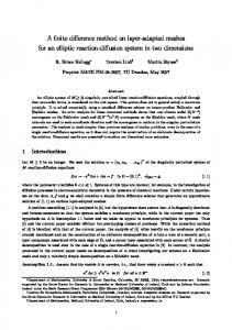
where I is an interpolation operator used to transfer information from the coarse grid to the fine grid. The first two steps are completely defined in the previous discussion, but one part of this algorithm deserves special attention: the calculation of the fine-grid boundary condition for the final local solve. Setting Fine-Grid Boundary Conditions for the Final Solve To set the boundary of a patch, we use both data from the local fine solutions and interpolants from the large coarse solution. We must be careful always to use the local data where they are available and yet not to add information twice by leaving the local effects in the coarse-grid data which we interpolate. The easiest way to keep track of all this is with a stencil. A sample interpolation stencil is shown in Fig. 1. We move the stencil around the sides of each patch such that its center row covers the projection of the boundary points which we wish to set. Coarse-grid data are interpolated from the nine coarse-grid points which lie under the stencil. Note that for accurate interpolation we need consistent data from all nine points. In Fig. 1, for example, we would subtract φ h,m,initial from the coarse-grid stencil values, but we would not subtract φ h,n,initial , since the stencil is not contained entirely by nH . We later add local data from φ h,m,initial , but not from φ h,n,initial , since those values were included in the coarse-grid interpolant.

FIG. 1.

An interpolation stencil as placed on the coarse grid.

36

BALLS AND COLELLA

FIG. 2.

An interpolation stencil as used to evaluate fine-grid values.

Figure 2 shows the fine-grid points we interpolate from the coarse-grid stencil. Note that stencils generally share the fine points furthest from the center with neighboring stencils. When multiple stencils can be used to evaluate a fine-grid point, we average all the values produced by the various stencils. We are able to construct an interpolant which is accurate to O(H 5 ) from our coarse stencil. Since we have subtracted all local information from our stencil values, φ H,stencil = φ H − φ H,m,initial , (58) m: mH ⊃ H,stencil

we have also made the coarse stencil data harmonic: L 9 φ H,stencil = L 9 φ H − L 9 φ H,m,initial = 0.

(59)

m: mH ⊃ H,stencil

We interpolate by constructing approximate derivatives and a Taylor series representation of a local solution. Since the coarse stencil values are harmonic, we are able to use a compact 3 × 3 stencil to compute sufficiently accurate approximations of the derivatives necessary as interpolation coefficients to guarantee that the interpolated results, φ h,stencil , are accurate to O(H 5 ) overall. Let us consider, for example, a top or bottom boundary, for which the fine-grid values of jx vary but j y remains constant. The difference approximations to the necessary derivatives are ∂ 4ψ ∂ 4ψ =− 2 2 4 ∂x ∂x ∂y 1 = − 2 4ψ jH − 2 ψ jHx +1, jy + ψ jHx −1, jy + ψ jHx , jy +1 + ψ jHx , jy −1 + ψ jHx +1, jy +1 H + ψ jHx +1, jy −1 + ψ jHx −1, jy +1 + ψ jHx −1, jy −1 + O(H 2 ), (60) ∂ 3ψ ∂ 3ψ = − ∂x3 ∂ x∂ y 2 1 H = + ψ jHx −1, jy −1 − ψ jHx +1, jy +1 − ψ jHx +1, jy −1 ψ 2H 3 jx −1, jy +1 + 2 ψ jHx +1, jy − ψ jHx −1, jy + O(H 2 ),

(61)


H 2 ∂ 4ψ ∂ 2ψ 1 H H H = − 2ψ + ψ + O(H 4 ), ψ −

+1, j −1, j j j x y x y j ∂x2 H2 12 ∂ x 4

37

(62)

and H 2 ∂ 3ψ ∂ψ 1 H + O(H 4 ), = ψ jx +1, jy − ψ jHx −1, jy − ∂x 2H 6 ∂x3

(63)

where the values of j refer to the indices of the coarse stencil. Note that the approximation (60) is needed for (62), and (61) is needed for (63). We use these approximations in a Taylor series approximation to interpolate fine-grid values: φ Nr h j+ j = I(φ H ) j = φ Hj + δh h

∂φ δ3 ∂ 3φ δ4 ∂ 4φ δ2 ∂ 2φ + O(H 5 ). + h 2 + h 3 + h ∂x 2 ∂x 6 ∂x 24 ∂ x 4

(64)

Here we still have j as the coarse-grid index. The index j h represents the displacement, in fine-grid spacing, from the projection of the center of the coarse stencil onto the fine grid. The distance δh is the quantity h| j h |. Finally, we add back the local fine-grid information to the interpolated data in the stencil: φ h,stencil = φ h,stencil +

φ h,m,initial .

(65)

h,g m: m ⊃ H,stencil

We copy these values into the appropriate boundary cells of φ h,l . Once we have traversed the boundaries of every patch and set the boundary conditions, we use multigrid to solve L 5 φ h,l = ρ h,l .

(66)

Our solution, φ h , is then a composite of the φ h,l calculated on each subdomain. Since our boundary condition sets coincident boundaries exactly the same, we do not need to worry about φ h being multivalued at the intersections of subdomains. We will later demonstrate that the combination of fine and coarse data which we used to set boundary conditions is accurate to O(h 2 ) + O(H 4 ) anywhere we wish to apply it. We need not set boundary values along the original subdomain boundaries: we could divide the original domain into a different set of patches, use the interpolation and correction as described to set the boundary conditions on the new patches, and expect the final solution to be just as accurate. Indeed, we could achieve the same overall accuracy by applying the stencil everywhere to generate fine-grid values. In many applications, our approach of setting boundary conditions for a final solve is preferable. With such a method, the error away from the boundaries of the subdomains is sufficiently smooth that one can apply difference operators to the solution to approximate, e.g., ∇φ, to O(h 2 ) accuracy. 3.2. Error Analysis of MLC The algorithm we have just presented divides a charge field ρ with support confined to

into several small charge fields ρ l defined on subdomains l . We can understand most of

38

BALLS AND COLELLA

the properties of this algorithm by looking at a simpler subproblem, such that the right-hand side, ρ, is a charge with bounded support on some smaller domain, ρ . Let us consider the application of our algorithm to this simpler problem. We subdivide the problem into patches such that a single patch, 0h , contains the support of ρ. Our solution is found in three steps. • First, solve L 9 φ h,0,initial = ρ h,0

(67)

h,g

on 0 with infinite domain boundary conditions. • Next, solve L 9φ H = R H

(68)

on H , the coarse domain covering the entire problem, with infinite domain boundary conditions. • Finally, set boundary conditions on each patch as φ

h,l

=

h,g

φ h,0,initial + I(φ H − φ H,0,initial ),

for boundary points in 0 ,

I(φ H ),

otherwise,

(69)

and solve a Poisson equation on each patch with the Dirichlet boundary conditions just set. To better understand our result, let us construct an auxiliary solution, the solution to L 9 φ¯ h = ρ h

(70)

on h with infinite domain boundary conditions. We have shown previously that φ¯ h and φ h,0,initial are accurate to O(h 2 ) on their domains. If we can show that the boundary conditions we set, (69), are accurate to O(h 2 ) as well, it follows that our algorithm is accurate to O(h 2 ) overall. It is sufficient to show φ¯ h − [φ h,0,initial + I(φ H − φ H,0,initial )] = O(h 2 ),

(71)

h,g

for all boundary points in 0 , and φ¯ h − I(φ H ) = O(h 2 ),

otherwise.

(72)

First, let us note that while φ¯ h and φ h,0,initial are both only accurate to O(h 2 ), by (38), they differ from one another by O(h 4 ); i.e., φ¯ h − φ h,0,initial = O(h 4 ).

(73)

Let us now define R˜ H =

L 9 (Sample H (φ¯ h )), outside 0H , 0,

in 0H .

(74)


39

R˜ H represents the error we make in our method by truncating R˜ H to be zero outside the correction radius. Note that φ H = Sample H (φ¯ h ) + (L 9 )−1 R˜ H + ξ B ,

(75)

where ξ B represents the error in the infinite domain boundary condition, which is O(H 4 ). h,g Since φ¯ h differs from a harmonic function by O(h 6 ) outside 0 (away from the support of ρ), we know L 9 (Sample H (φ¯ h )) = O(H 6 )

(76)

R˜ H = O(H 6 ).

(77)

φ H = Sample H (φ¯ h ) + O(H 4 ),

(78)

outside 0H , and therefore

Thus (75) becomes

h,g

and the resulting error estimate for boundary points within 0 is ξ h,BC = O(h 4 ) + O(H 4 ).

(79)

h,g

For points outside 0 , we note again that φ H = Sample H (φ¯ h ) + O(H 4 )

(80)

and that φ¯ h is harmonic in this region. Therefore φ H differs from a harmonic function by terms that are O(H 4 ), and the far-field interpolated values obtained in (69) differ from φ¯ h by O(H 4 ). The resulting composite solution, then, is accurate to O(H 4 ) + O(h 2 ). As long as the refinement ratio is chosen correctly, such that the O(H 4 ) and O(h 2 ) terms are comparable, we can guarantee an accuracy of O(h 2 ) over the entire domain h . 3.3. Parallel Implementation The implementation of this algorithm in parallel is fairly straightforward. Given a parallel machine with Nprocs processors we assign patches associated with the fine grids of the domain decomposition cyclically to each of the processors. Generally we use Nprocs equal to exactly the number of patches in the decomposition. Both the initial local infinite domain Poisson solves and the final multigrid solves on the fine grids can be performed in parallel without any communication among the processors during those phases of the computation. In a fashion similar to Baden’s parallel implementation of the MLC [4], we have chosen to construct the global coarse-grid representation of both the right-hand side and the solution on each processor. Since the global coarse grid requires fewer grid points than any individual fine grid, this overhead is small both in terms of memory and computation required. To build the global coarse representation, all the processors need to broadcast the coarse-grid righthand sides for each of their patches to all the other processors. This communication step creates the global coarse right-hand side necessary for the global infinite domain Poisson

40

BALLS AND COLELLA

solve. All the processors then perform that same solve, after which every processor has a copy of the coarse-grid field necessary for the final phase of the computation. The only other communication necessary is the communication among patches to correct the interpolation of the fine-grid boundary conditions. This communication occurs between processors which control neighboring patches and only points along the boundary are communicated, so the communication requirement for this step is rather small. 3.4. The Relationship among Patches, Refinement Ratio, and Problem Size We would like for our algorithm to be scalable on a parallel machine. To ensure scalability, we need to consider the effect of the parts of the algorithm which are performed as serial rather than parallel computations. In our algorithm, the global coarse-grid infinite domain solve is the only serial calculation. We need to show that this part of the calculation can be scaled such that it does not limit the parallel performance of the algorithm as a whole. Let us consider a problem domain represented on a fine grid of dimensions [0, N ] × [0, N ]. We divide the domain into N p patches in each direction for a total of N p × N p patches. We represent the global coarse data on a grid of dimensions [0, N C ] × [0, N C ]. The ratio of coarse-grid spacing to fine-grid spacing is the refinement ratio Nr = NNC . Scalability requires that the work done on the global coarse solve be proportional to the work done on each patch. The work done on the global coarse solve is proportional to the 2 2 size of the coarse grid: O((N C )2 ) = O( Nn 2 ). The work per patch is O( NN 2 ). This implies that r p we need a refinement ratio Nr proportional to the number of patches in each direction N p . Now we must consider whether it is feasible to increase the refinement ratio as we increase the number of patches. We expect our global solve to be accurate to O(H 4 ) while the overall method is only accurate to O(h 2 ). This implies a relationship between the refinement ratio and size of the problem since Nr = Hh . We need (Nr h)4 ∝ h 2 ,

(81)

1 , h2

(82)

Nr4 ∝ or

Nr2 ∝ N .

(83)

Combining this relationship with the relationship between patches and refinement ratio, we have Nr2 ∝ N p2 ∝ N .

(84)

If we hold to these relationships, the algorithm should exhibit both good parallel performance and O(h 2 ) accuracy overall. 3.5. Computational Overhead To analyze the conditions under which our method is most attractive, we need to estimate the overhead incurred in performing this type of domain decomposition. Multigrid typically requires O(M log M) work to calculate a solution to Poisson’s equation on a grid of M


41

points. For the purposes of this analysis, we will refer to this amount of work as M work units, ignoring the log term. Note that this simplification favors large single grids over domains decomposed into smaller grids. First, let us consider the single-grid infinite domain problem. The solution for a domain

h,0 requires first a multigrid solution on an intermediate domain, h,initial , and then a solution on a larger domain, h . For good accuracy we need h to be at least 10% larger than h,0 in each direction. This requirement results in an overall size of 1.2N × 1.2N = 1.44N 2 . The size of h,initial is then 1.1N × 1.1N = 1.21N 2 . The two multigrid solutions combined require 1.44N 2 + 1.21N 2 work units. The potential calculation also requires O(N 2 ) work, but the cost is small compared to the multigrid solutions, and we will not consider this portion of the work. The work required for the single-grid solution is then at least 2.65N 2 work units. For the parallel solution, our method involves three large steps: first, we solve a number of independent problems with infinite domain boundary conditions; then, after aggregating coarse data, we solve the coarse-grid problem for the entire domain with infinite domain boundary conditions; and finally, after setting accurate boundary conditions, we solve local fine-grid problems with Dirichlet boundary conditions. Communication steps are required between the major computational steps, but we are interested in estimating only the computational overhead here. For a problem of size N × N , we use N p × N p processors and a refinement ratio of Nr to determine the coarse-grid spacing. We require N p2 ∝ Nr2 ∝ N for accuracy reasons, so let us take √ Np = a N (85) and

√ Nr = b N .

(86)

For the first step of our algorithm, we solve infinite domain boundary condition problems of size ( NNp + 4Nr )2 on each of our N p2 independent fine grids. These solutions, as in the single-grid case, require two separate multigrid solutions. The first set of solutions, on intermediate grids of size ( NNp + 2Nr )2 , requires

2 N + 2Nr Np √ 2 √ N 2 =a N + 2b N a

W1a = N p2

= (1 + 4ab + 4(ab)2 )N 2 work units, and the second set of solutions requires 2 N W1b = N p2 + 4Nr Np √ 2 √ N 2 =a N + 4b N a = (1 + 8ab + 16(ab)2 )N 2 work units.

(87)

(88) (89)

(90)

(91) (92)

42

BALLS AND COLELLA

Taken together, again ignoring the cost of the potential calculation, we find that the first step in our method requires W1 = (2 + 12ab + 20(ab)2 )N 2 work units.

(93)

It is important to note, however, that the work required for this step cannot be less than 2.65N 2 work units: the individual infinite domain solutions are subject to the same constraints on domain sizes as in the single-grid solution, and thus our method requires at least as much work as the single-grid solve. We have chosen to implement the second step of our algorithm, the global coarse-grid solution with infinite domain boundary conditions, as a calculation which is replicated across all the processors. Thus our N p2 = a 2 N processors each solve a problem of size ( NNr )2 = bN2 . These problems have the same overhead as a single-grid calculation, so we can estimate the work for this second stage as W2 = 2.65

a2 2 N work units. b2

(94)

Finally, we need to solve the independent problems on each domain with Dirichlet boundary conditions. The work required for this step is simply W3 = N 2 work units.

(95)

Taken together, we see that the total work must be at least 3.65N 2 work units. We can ensure that the work is not much greater than that, however. Choosing Nr and N p such that 1 ba ≤ 16 is sufficient to ensure that W1 < 2.83N 2 work units. Choosing Nr and N p such b that a ≥ 4 ensures that W2 ≤ 0.17N 2 work units. Together, these conditions ensure that the total work is less than 4N 2 work units. In terms of N p , Nr , and N , the conditions for small computational overhead are expressed as Nr ≤

1√ N 2

(96)

Np ≤

1 Nr . 4

(97)

and

These conditions imply that the smallest problem we can solve with this little overhead is a 65 × 65 problem on a single patch with Nr = 4. The smallest problem we can solve in parallel with such a small amount of computational overhead is a 257 × 257 problem on 2 × 2 patches with Nr = 8. Using these estimates to calculate theoretical speed-up, with a 7% overhead of serial computation for the global coarse-grid solution, we would expect our solution of the 257 × 257 problem on four processors to be 2.65 times as fast as the single-grid calculation. These constraints do not seem excessive since the algorithm is specifically designed for solving large problems on large parallel machines and since we have removed almost all the communication overhead required by a standard multigrid method.


43

4. RESULTS

We have implemented versions of our algorithm in order to test our claims. Computer programs were written in two separate programming environments designed for building parallel algorithms for scientific computations: KeLP and Titanium. KeLP, designed and written by Baden, Fink, and Kohn [5, 9], is a C++ library that provides a large number of useful features both for parallel programming and for scientific computing. KeLP provides for interfaces between high-level C++ descriptions of the data structures and lower level numerical algorithms, implemented in Fortran. This division allows the user to take advantage of the performance provided by Fortran compilers as well as the abstractions supplied by the C++ language. Titanium [17] is a dialect of Java developed for parallel scientific applications. The language has a SPMD model of parallel execution and has built-in abstractions which are useful for scientific applications. The Titanium compiler aggressively optimizes many of the most common routines in scientific computations, such as loops over two- or three-dimensional arrays. The performance of the Titanium code is slightly slower than that of the KeLP implementation for our algorithm, but since the Titanium code was easier to write and modify, it proved more amenable to algorithm development and testing. All the results presented here are generated by code written in Titanium. Timing tests were run on the IBM SP2 at the San Diego Supercomputing Center. Additional results and comparisons including data for the KeLP implementation can be found in [7]. One of the benefits of solving the Poisson equation is that we can easily create test problems for which exact analytical solutions can be calculated directly. In such cases, we are able to measure the error in our computed solution by comparing it with the exact solution. We also use test problems for which the exact solution is not known. In these cases we perform Richardson error estimation, using a series of increasingly refined solutions, comparing each to the next finer. In all cases, we can calculate a convergence rate for our method from norms of the error estimates as the grid is refined. There are several properties that we seek to demonstrate about our algorithm. First, we show that our algorithm is accurate to O(h 2 ). Specifically, we show that the solution converges as predicted when the problem is scaled appropriately, i.e., when the refinement ratio, Nr , and the number of patches (in each direction), N p , are inversely proportional to the square root of the grid spacing, h. In addition, we show that our algorithm produces more accurate results than a single infinite domain boundary condition solution on coarse-grid data with Mehrstellen preconditioning (29). Finally, we measure the performance of the algorithm on a parallel machine, testing communication costs and speedup. 4.1. The Test Problems We have two similar test problems for which we can construct solutions. Both problems have radially symmetric charge distributions. The first charge distribution is very smooth:

ρ=

 

r R0

 0,

−

r2 4 , R02

r < R0 , r ≥ R0 .

(98)

44

BALLS AND COLELLA

This charge can be integrated directly to produce an exact solution:  2 a8 7 6 5 a4 r 100 − 4a + 6a − 4a + 36  81 64 49   1 φ= +R02 10 − 49 + 68 − 47 + 16 log(R0 ), r < R0 ,    2 1 R0 10 − 49 + 68 − 47 + 16 log(r ), r ≥ R0 .

(99)

Our second test problem includes a tunable wavenumber component. This is useful to demonstrate how methods perform on charges with a high wavenumber which can only be resolved on fine grids. This second charge is defined as   sin(wr ) r 2 − r 22 2 , r < R0 , R0 R0 ρ= (100)  0, r ≥ R0 . We define w to be 2mπ , where m is a positive integer. The solution for this right-hand side R0 can be represented as φ=

φinterior , r < R0 , φexterior , r ≥ R0 ,

(101)

where the interior and exterior solutions are defined as 137 cos(2wr ) − 1 47a 2 − 52a + 11 φinterior = − w2 64(w R0 )4 32(w R0 )2 cos(2wr ) (a 4 − 2a 3 + a 2 ) w2 8 sin(2wr ) 77a − 50 9a 3 − 14a 2 + 5a + − w2 32(w R0 )3 16wr 3 cos(2wr ) 15 + − dr − log(r ) r 16w 4 R02 16w 6 R04 3 sin(2wr ) r4 r5 r6 + dr + − + r 4w 5 R03 32R02 25R03 72R04 37R02 R02 log(R0 ) 45 − + 1+ 4 4 7200 120 w R0 +

(102)

and φexterior

R02 log(r ) 45 = 1+ 4 4 . 120 w R0

(103)

We are unable to write down a closed-form solution for this right-hand side because it ) ) involves integration of terms such as sin(r and cos(r . We generate integrals of these terms r r by numerical techniques, such as Taylor expansion near the singularity at the origin and Richardson–Romberg integration elsewhere [3]. These numerical approximations provide much higher order accuracy and are calculated with steps much smaller than the grid spacing used in our algorithm so that we can ensure that they are far more accurate than the O(h 2 ) we


45

expect from our algorithm. This extra accuracy is essential, since we compare the solutions calculated by our finite difference methods to this solution. We have a third test problem for which no analytical solution is available. This charge distribution is a variation on the tunable wavenumber test problem just described. The charge distribution varies in θ , as well as r . We define this charge as ρ=

  sin wr∗ R

r R∗

−

r2 R ∗2

2

, r < R∗,

 0,

r ≥ R∗,

(104)

where w is defined as before and R ∗ is defined as R∗ =

R0 cos(6θ) + 3 . 4

(105)

The effect of the R ∗ term is to create lobes out from the center of the charge. Our particular choice of R ∗ creates a six-lobed charge field. Since no analytical solution is available for this charge distribution, Richardson error estimation must be used to study the convergence of the solution in this case. 4.2. Validation of Far-Field Error Estimates We show by numerical experiments that our analysis in Section 3.2 is correct. We are interested in confirming our estimates in (76) and (77), specifically that R˜ H = L 9 (Sample H (φ h )) = O(H 6 ),

(106)

in the far field. Recall that this R˜ H is a measure of the error we make in our algorithm by truncating the far-field charge to zero when constructing the coarse charge field for the global coarse solve. To verify this assertion, we use a test problem in which the charge has compact support, limited to a fraction of the solution domain. The charge that we use for these tests is given 1 by (98), centered at ( 14 , 14 ), with a radius R0 = 16 . The problem is solved on the domain 2 [0, 1] × [0, 1] in . Figure 3 shows this far-field truncation error in the coarse-grid representation of the charge for a fine-grid domain of size 65 × 65. The curve fits in this truncation error plot are represented by H6 R˜ H = 3.64 × 10−6 8 , |x |

(107)

where H is the grid spacing used for the coarse-grid Laplacian operator. This relationship implies that the coarse-grid truncation error is O(H 6 ). The variation of R˜ H as |x 1|8 is also expected since the coefficients of O(H 6 ) terms in the error estimate are eighth derivatives of the solution, and the solution is harmonic in the far field. Since the harmonic Green’s function is proportional to log(|x |), the eighth derivatives of a harmonic function are then O( |x 1|8 ). To demonstrate that the error is a function only of coarse-grid spacing and distance from the center of the charge, we have plotted the results for a 65 × 65 grid with Nr = 2, a

46

BALLS AND COLELLA

FIG. 3.

Far-field coarse truncation error for a 65 × 65 fine grid.

129 × 129 grid with Nr = 4, and a 257 × 257 grid with Nr = 8 in Fig. 4. For each of these 1 problems, the coarse-grid spacing remains a constant H = 32 , and all the data lie along a single line, independent of the fine-grid spacing used to solve the Poisson problem. 4.3. Mesh Refinement Studies for the Full Algorithm We now demonstrate by mesh refinement studies that our method produces results that are accurate to O(h 2 ) as the solution grid is refined and that the additional error induced by the domain decomposition is small, relative to the intrinsic solution error from a five-point discretization of Poisson’s equation. Accuracy for a High-Wavenumber Charge We use two test cases with high-wavenumber components to gauge the performance of our method on nonsmooth charge distributions. It is difficult to assess accuracy of a

FIG. 4.

Coarse-grid truncation errors for various fine-grid problems with a constant coarse-grid spacing.

47


TABLE I Error Norms and Convergence Rates for a Problem with a High-Wavenumber Charge Distribution, Solved with Various Grid Sizes, Numbers of Patches, and Refinement Ratios Error norms

Convergence rates

Grid size

Np

Nr

|error|max

|error|2

|error|max

|error|2

129 × 129 129 × 129 129 × 129 129 × 129 257 × 257 257 × 257 257 × 257 257 × 257 513 × 513 513 × 513 513 × 513 513 × 513

1 1 2 2 2 2 4 4 2 2 4 4

2 4 4 8 4 8 8 16 4 8 8 16

4.42e-7 4.41e-7 4.91e-7 4.83e-7 8.61e-8 8.51e-8 8.25e-8 7.23e-8 2.02e-8 2.01e-8 1.96e-8 1.67e-8

9.21e-8 9.18e-8 1.03e-7 1.00e-7 2.18e-8 2.13e-8 2.02e-8 1.77e-8 5.32e-9 5.26e-9 5.05e-9 4.12e-9

2.22 2.23 2.32 2.42

2.06 2.06 2.18 2.30

method on high-wavenumber charges in terms of a standard convergence study: as the grid is refined, the problem becomes relatively more smooth. Therefore, for these tests, we restrict ourselves to three grid sizes: 129 × 129, 257 × 257, and 513 × 513. The results for the radially symmetric test problem are shown in Table I. For this set of test problems, the charge was defined by (100), with R0 = 0.42 and m = 15. These parameters result in 30 periods over the radius of the charge, or approximately 1.8 grid points per period on the 129 × 129 grid, which is insufficient to resolve the solution. The 257 × 257 grid has adequate resolution, and the 513 × 513 grid is well resolved, with over 7 grid points per period. The convergence rates reported in Table I are based on comparing the 513 × 513 grid errors with the errors on the corresponding grids of size 129 × 129. These may be questionable since the 129 × 129 grid is underresolved, but calculating the convergence based on the 513 × 513 and 257 × 257 grids gives O(h 2 ) convergence uniformly as well. An error plot for this problem calculated on a 257 × 257 grid with N p = 2 and Nr = 8 is shown beside an error plot for the same problem solved on a single 257 × 257 grid in Fig. 5. The plots are very similar, and, equally important, the domain decomposition algorithm does not add any strong discontinuities to the error. The error norms for the single-grid solutions are shown in Table II. To be fair, however, we should also compare our results with results from an infinite domain solver which uses Mehrstellen preconditioning: we need to demonstrate that a much simpler, single-grid solution on a much coarser grid could not produce equally accurate results. In Table III we juxtapose the previous results from our algorithm with results from an infinite domain solution using Mehrstellen preconditioning (29). The MLC algorithm is used with the fine- and coarse-grid sizes as noted in the table; the corresponding single-grid infinite domain Poisson solution with Mehrstellen preconditioning is performed on a grid with the coarse spacing. Note that in some cases, there are multiple values of N p for the grid sizes and refinement ratios indicated in the table: in every such case we have chosen the result which reflects the largest errors for our algorithm. We see that for any Nr we choose, our method is more accurate than any single-grid solution with Mehrstellen precondition-

48

BALLS AND COLELLA

FIG. 5. On the left, error for a high-wavenumber, radially symmetric charge covering most of the solution domain, a 257 × 257 grid, with N p = 2 and Nr = 8; on the right, the error resulting when the same problem is solved on a single 257 × 257 grid.

ing on the corresponding coarse-grid domain. Until the problem is sufficiently resolved on the grid, the benefits of a higher order method with Mehrstellen preconditioning are not realized. Accuracy for an Extremely Large Problem The ability to solve large problems is one of the main reasons for developing parallel algorithms. Unfortunately, as problem sizes get larger and charge distributions get more complicated, it becomes more difficult to study convergence of the solution. Here we solve a rather complicated problem on grids of size 513 × 513, 1025 × 1025, and 2049 × 2049, testing the accuracy of our solutions on the 513 × 513 and 1025 × 1025 grids by using Richardson error estimation. The charge distribution for this large problem is the superposition of three separate high-wavenumber charge fields and a smooth, radially symmetric field. Two of the highwavenumber charge fields are six-lobe charge fields as defined by (104); the third is a radially symmetric charge field defined by (100). The smooth, radially symmetric charge field is defined by (98). The problem domain is defined on [0, 1] × [0, 1]. One six-lobe charge with m = 6 and R0 = 0.25 is placed at (0.35, 0.3). A second six-lobe charge with m = 4 and R0 = 0.18 is placed at (0.75, 0.8). The high-wavenumber, radially symmetric charge has m = 18 and R0 = 0.38 and is placed at (0.6, 0.4). The smooth, radially symmetric charge is placed at (0.4, 0.5) and also has R0 = 0.38. Error norms for this large problem are listed in Table IV: again the method exhibits O(h 2 ) accuracy. TABLE II Error Norms for a Single-Grid Solution of the High-Wavenumber Problem Grid size

|error|max

|error|2

129 × 129 257 × 257 513 × 513

4.92e-7 8.62e-8 2.02e-8

1.19e-7 2.42e-8 5.83e-9

49


TABLE III Comparison of Maximum Error Norms for a Single Coarse-Grid Solution of the High-Wavenumber Problem, Utilizing Mehrstellen Preconditioning, to Error Norms for MLC Fine size

Nr

Coarse size

MLC |error|max

Mehrstellen |error|max

129 × 129 129 × 129 257 × 257 257 × 257 513 × 513 513 × 513 513 × 513

2 4 4 8 4 8 16

65 × 65 33 × 33 65 × 65 33 × 33 129 × 129 65 × 65 33 × 33

4.42e-7 4.91e-7 8.61e-8 8.51e-8 2.02e-8 2.01e-8 1.67e-8

1.13e-5 5.97e-4 1.13e-5 5.97e-4 1.75e-7 1.13e-5 5.97e-4

Ratio:

MLC Mehrstellen

3.9e-2 8.2e-4 7.6e-3 1.4e-4 1.2e-1 1.8e-3 2.8e-5

TABLE IV Error Norms for a Very Large, High-Wavenumber Problem

FIG. 6.

Grid size

Np

Nr

|error|max

513 × 513 1025 × 1025

2 4

8 16

2.97e-8 6.47e-9

Error for a high-wavenumber charge, solved on a 1025 × 1025 grid with 16 patches and Nr = 16.

50

BALLS AND COLELLA

A plot of the error on the 1025 × 1025 grid appears in Fig. 6. It is possible to see faint traces along the domain boundaries in this plot. These artifacts are very small in magnitude compared to the intrinsic error due to the five-point discretization of the Poisson equation. 4.4. Parallel Timing We would like to confirm experimentally that our algorithm scales well as the number of processors is increased. There are many different measures of parallel speedup, depending on the type of problem being solved. For some problems multiple processors are used in order to take advantage of parallelism inherent in the problem. For such problems, one hopes to compute solutions to the same problem in an amount of time inversely proportional to the number of processors available. For another class of problems, however, multiple processors are needed because the data are too numerous to fit in the memory associated with a single processor. For these types of problems, scaled speedup is a more appropriate measure of parallel performance. In scaled speedup tests, the size of the problem is scaled in proportion to the number of processors, and one hopes that the time to compute solutions remains constant even as the problem size increases. Our algorithm is designed for scaled speedup. As discussed in Section 3.5, our method introduces some degree of computational overhead even when solving Poisson’s equation with infinite domain boundary conditions. If our method were used instead to solve problems with simpler Dirichlet boundary conditions, the overhead would be an even greater factor. As a result, single-grid methods are preferable when problems are small enough to fit on a single processor. As problem sizes grow, however, and parallelism is necessary, the scaled speedup provided by our algorithm becomes more attractive. We constructed series of test problems for which the amount of computation required per processor remains approximately constant. For this performance study, we expect the wallclock time required to be nearly constant as the problem sizes and number of processors increase. The amount of computation required per processor depends on both the local fine-grid patch sizes and the global coarse-grid size. Therefore, as we increase the overall problem size, N , we need to increase both the refinement ratio, Nr , and the number of patches in each direction, N p . Three series of test problems were run on 1 to 16 processors. The parameters for these series are shown in Tables V–VII. The results of the first groups of scaled speedup tests, shown in Fig. 7, are very near what we would expect. The three series lie nicely along horizontal lines. In fact, the deviations from perfectly horizontal lines can be explained almost entirely by variations in the total number of multigrid iterations required. We are not only interested in the total time required to compute solutions, however. We are also interested in the fraction of time spent communicating data among the processors. TABLE V Scaled Speedup Test: Series 1 Total size

Patches

Refinement ratio

Local fine size

Global coarse size

129 × 129 257 × 257 513 × 513

1×1 2×2 4×4

4 8 16

129 × 129 129 × 129 129 × 129

33 × 33 33 × 33 33 × 33

51


TABLE VI Scaled Speedup Test: Series 2 Total size

Patches

Refinement ratio

Local fine size

Global coarse size

257 × 257 513 × 513 1025 × 1025

1×1 2×2 4×4

4 8 16

257 × 257 257 × 257 257 × 257

65 × 65 65 × 65 65 × 65

TABLE VII Scaled Speedup Test: Series 3 Total size

Patches

Refinement ratio

Local fine size

Global coarse size

513 × 513 1025 × 1025 2049 × 2049

1×1 2×2 4×4

4 8 16

513 × 513 513 × 513 513 × 513

129 × 129 129 × 129 129 × 129

TABLE VIII Communication Costs for a Series with O(h2 ) Convergence Problem size

Patches

Nr

Communication time (s)

Percent of total

257 × 257 513 × 513 513 × 513 1025 × 1025 1025 × 1025 2049 × 2049

2×2 2×2 4×4 2×2 4×4 4×4

8 8 16 8 16 16

0.081 0.17 0.16 0.31 0.30 0.54

1.5 1.1 2.5 0.57 1.7 0.96

FIG. 7.

Timing results for a scaled speedup test.

52

BALLS AND COLELLA

The communication overhead for our algorithm, shown in Table VIII, is very small and never more than 2.5% of the total time for the method.

5. CONCLUSIONS

We developed a parallel finite difference algorithm for the computation of the solution to the Poisson equation with infinite domain boundary conditions. Our algorithm produces results accurate to second order for a wide range of problems. The errors in the computed solution are almost entirely a function of fine-grid spacing. The division of the problem into subdomains produces additional errors at the boundaries which are small in magnitude compared to the errors on the interiors of the subdomains. In fact, the overall errors for solutions calculated by our method are comparable to those produced by a standard second-order single-grid solver. The accuracy of the solution is not significantly degraded even for very coarse global grids. We have found that it is possible to use coarse-grid spacings large enough that the coarse-grid solve represents only about a 2–7% increase in the total number of floating point operations. The amount of communication required is small. Time spent in communication represents no more than 2.5% of the total time required to compute a solution for the Titanium implementation of the algorithm running on the IBM SP2 at the San Diego Supercomputer Center. Since both our parallel computational overhead costs and our communication requirements are small, we expect our algorithm to exhibit very good parallel scaling. We find that our program does obtain linear speedup on the SP2. An important extension of this research will be the development of the three-dimensional analogue of this algorithm. Unlike many other approaches, which become much more complex or much less efficient in the transition from two to three dimensions, our algorithm should remain fairly simple and largely unchanged. The most significant change required has to do with the potential calculation for the infinite domain solve: a straightforward extension of our method to three dimensions would result in a method which required O(N 4 ) work to compute the boundary charge on a grid of N 3 points. This method would be unacceptable since all other phases of the computation would be expected to require O(N 3 log√N 3 ) work at most. Projecting the potential onto a coarser outer grid, of spacing H = O( h), would reduce the work required to O(N 3 ), again, though, and O(H 8 ) interpolation on the outer grid to set the boundary condition would be tedious, but not computationally expensive. Another important addition to our algorithm would be the introduction of alternative boundary conditions. Many real-world problems require Dirichlet, Neumann, or some sort of mixed boundary conditions for which our algorithm is not currently designed to handle. One approach to supplying alternative boundary conditions to problems such as these uses image charges. An example of this approach is described by Baden and Puckett [6]. It would also be interesting to look at making the algorithm adaptive: we have seen that the accuracy of our method depends very weakly on the coarse-grid spacing, and it should be possible to use coarser local grids on patches with low-wavenumber charge distributions. Adaptivity such as this would require us to look into load-balancing issues much more carefully, however.


53

ACKNOWLEDGMENTS We thank Scott Baden for his help in implementing early versions of this work in KeLP. We thank the Titanium group at the University of California, Berkeley, for their help in analyzing and improving the Titanium version of our code and especially Katherine Yelick for her advice in designing parallel code. Support for this work was provided by the following grants and fellowships: National Science Foundation Graduate Fellowship Program, National Science Foundation; The Berkeley Fellowship, University of California at Berkeley; Adaptive Numerical Methods for Partial Differential Equations, US Department of Energy Mathematical, Computing, and Information Sciences Division, Grant DE-FG03-94ER25205; and Computational Fluid Dynamics and Combustion Dynamics, US Department of Energy High-Performance Computing and Communications Grand Challenge Program, Grant DE-FG03-92ER25140. This work was supported in part by the Advanced Research Projects Agency of the Department of Defense under Contract F30602-95-C-0136. The information presented here does not necessarily reflect the position or the policy of the Government and no official endorsement should be inferred.

REFERENCES 1. A. S. Almgren, T. Buttke, and P. Colella, A fast adaptive vortex method in three dimensions, J. Comput. Phys. 113, 177 (1994). 2. C. R. Anderson, A method of local corrections for computing the velocity field due to a distribution of vortex blobs, J. Comput. Phys. 62, 111 (1986). 3. B. M. Ayyub and R. H. McCuen, Numerical Methods for Engineers (Prentice Hall, Upper Saddle River, NJ, 1996). 4. S. B. Baden, Run-Time Partitioning of Scientific Continuum Calculations Running on Multiprocessors, Ph.D. thesis (University of California, Berkeley, 1987). 5. S. B. Baden, Software infrastructure for non-uniform scientific computations on parallel processors, Appl. Comput. Rev. 4, 7 (1996). 6. S. B. Baden and E. G. Puckett, A fast vortex method for computing 2d viscous flow, J. Comput. Phys. 91, 278 (1990). 7. G. T. Balls, A Finite Difference Domain Decomposition Method Using Local Corrections for the Solution of Poisson’s Equation, Ph.D. thesis (University of California, Berkeley, 1999). 8. L. Collatz, The Numerical Treatment of Differential Equations, 3rd ed. (Springer-Verlag, New York, 1966). 9. S. J. Fink, S. B. Baden, and S. R. Kohn, Efficient run-time support for irregular block-structured applications, J. Parallel Distributed Comput. 50, 61 (1998). 10. L. Greengard and J. Y. Lee, A direct adaptive solver of arbitrary order accuracy, J. Comput. Phys. 125, 415 (1996). 11. L. Greengard and V. Rokhlin, A fast algorithm for particle simulations, J. Comput. Phys. 73, 325 (1987). 12. L. Greengard and V. Rokhlin, A new version of the fast multipole method for the Laplace equation in three dimensions, Acta Numerica 6, 229 (1997). 13. R. A. James, The solution of Poisson’s equation for isolated source distributions, J. Comput. Phys. 25, 71 (1977). 14. K. Lackner, Computation of ideal MHD equilibria, Comput. Phys. Commun. 12, 33 (1976). 15. B. F. Smith and O. B. Widlund, A domain decomposition algorithm using a heirarchical basis, SIAM J. Sci. Stat. Comput. 11, 1212 (1990). 16. J. Strain, Fast potential theory. II. Layer potentials and discrete sums, J. Comput. Phys. 99, 251 (1991). 17. K. Yelick, L. Semenzato, G. Pike, C. Miyamoto, B. Liblit, A. Krishnamurthy, P. Hilfinger, S. Graham, D. Gay, P. Colella, and A. Aiken, Titanium: A high-performance Java dialect, Concurrency—Practice and Experience, Java Special Issue (1998).