A Comparison Study on Rule Extraction from Neural Network

Hindawi Applied Computational Intelligence and So Computing Volume 2018, Article ID 4084850, 20 pages https://doi.org/10.1155/2018/4084850

Research Article A Comparison Study on Rule Extraction from Neural Network Ensembles, Boosted Shallow Trees, and SVMs Guido Bologna

1,2

and Yoichi Hayashi3

1

Department of Computer Science, University of Applied Sciences and Arts Western Switzerland, Rue de la Prairie 4, 1202 Geneva, Switzerland 2 Department of Computer Science, University of Geneva, Route de Drize 7, 1227 Carouge, Switzerland 3 Department of Computer Science, Meiji University, Tama-ku, Kawasaki, Kanagawa 214-8571, Japan Correspondence should be addressed to Guido Bologna; [email protected] Received 27 July 2017; Revised 17 November 2017; Accepted 4 December 2017; Published 9 January 2018 Academic Editor: Erich Peter Klement Copyright © 2018 Guido Bologna and Yoichi Hayashi. This is an open access article distributed under the Creative Commons Attribution License, which permits unrestricted use, distribution, and reproduction in any medium, provided the original work is properly cited. One way to make the knowledge stored in an artificial neural network more intelligible is to extract symbolic rules. However, producing rules from Multilayer Perceptrons (MLPs) is an NP-hard problem. Many techniques have been introduced to generate rules from single neural networks, but very few were proposed for ensembles. Moreover, experiments were rarely assessed by 10-fold cross-validation trials. In this work, based on the Discretized Interpretable Multilayer Perceptron (DIMLP), experiments were performed on 10 repetitions of stratified 10-fold cross-validation trials over 25 binary classification problems. The DIMLP architecture allowed us to produce rules from DIMLP ensembles, boosted shallow trees (BSTs), and Support Vector Machines (SVM). The complexity of rulesets was measured with the average number of generated rules and average number of antecedents per rule. From the 25 used classification problems, the most complex rulesets were generated from BSTs trained by “gentle boosting” and “real boosting.” Moreover, we clearly observed that the less complex the rules were, the better their fidelity was. In fact, rules generated from decision stumps trained by modest boosting were, for almost all the 25 datasets, the simplest with the highest fidelity. Finally, in terms of average predictive accuracy and average ruleset complexity, the comparison of some of our results to those reported in the literature proved to be competitive.

1. Introduction The explanation of neural network responses is essential for their acceptance. As an example, physicians cannot trust any model without any form of enlightenment. An intuitive way to give insight into the knowledge embedded within neural network connections and neuron activation is to extract symbolic rules. However, producing rules from Multilayer Perceptrons (MLPs) is an NP-hard problem [1]. In the context of classification, the format of a symbolic rule is given as follows: “if tests on antecedents are true then class 𝐾,” where “tests on antecedents” are in the form 𝑥𝑖 ≤ 𝑡𝑖 or 𝑥𝑖 ≥ 𝑡𝑖 , with 𝑥𝑖 as an input variable and 𝑡𝑖 as a real number. Class 𝐾 designates a class among several possible classes. The definition of the complexity of the extracted rules is often described with two parameters: number of rules and

number of antecedents per rule. Rulesets of low complexity are preferred compared to those with high complexity, since at first sight fewer rules and fewer antecedents are better understood. Another reason of preference is that rule bases with lower complexity also reduce the risk of overfitting on new data. Nevertheless, Freitas clarified that the comprehensibility of rules is not necessarily related to a small number of rules [2]. He proposed a new measure denoted as prediction-explanation size, which strongly depends on the average number of antecedents per rule. Another measure of rule transparency is consistency. Specifically, an extracted ruleset is deemed to be consistent if, under different training sessions, the rule extraction algorithm produces rulesets which classify samples into the same classes. Finally, a rule is redundant if it conveys the same information or less general information than the information conveyed by another rule.

2

Applied Computational Intelligence and Soft Computing

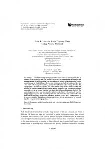
An important characteristic of rulesets is whether they are ordered or not. Ordered rules correspond to the following: if tests on antecedents are true then . . ., else if tests on antecedents are true then . . ., . . ., else . . . In unordered rules “else if” is replaced again by “if tests on antecedents are true then conclusion.” Thus, a sample can activate more than a rule. Long ordered rulesets are difficult to understand since they potentially include many implicit antecedents; specifically, those negated by “else if.” Generally, unordered rulesets present more rules and antecedents than ordered ones, since all rule antecedents are explicitly provided, thus being more transparent than ordered rulesets. Each rule of an unordered ruleset represents a single piece of knowledge that can be examined in isolation, since all antecedents are explicitly given. With a great number of unordered rules, one would try to accurately understand the meaning of each rule with respect to the data domain. Getting the global picture could take a long time; nevertheless, one could be interested only in some parts of the whole knowledge, for instance, those rules with the highest number of covered samples. The Discretized Interpretable Multilayer Perceptron (DIMLP) represents a special feedforward neural network architecture from which crisp symbolic rules are extracted in polynomial time [3]. This particular Multilayer Perceptron (MLP) model can be used to learn any classification problem, and rule extraction is also performed for DIMLP ensembles. Furthermore, special DIMLP architectures were also defined to produce fuzzy rules [4]. Decision trees are widely used in Machine Learning. They represent transparent models because symbolic rules are easily extracted. However, when they are combined in an ensemble rule, extraction becomes harder [5]. Here, we propose generating rules from ensembles of shallow decision trees with the help of DIMLP ensembles. In practical terms, each rule extracted from a tree is inserted into a single DIMLP network; then, all the rules generated from a tree ensemble are represented by a DIMLP ensemble. Finally, rule extraction is performed to obtain a ruleset representing the knowledge embedded within the decision tree ensemble. Because of the No Free Lunch Theorem no model is better than any other, in general [6]. Hence, if a connectionist model is more accurate than a direct rule learner such as RIPPER [7], then it is worth extracting rules to understand the classifications, even if this involves extra computing time. Authors who generated rules from single neural networks or Support Vector Machines (SVMs), very rarely assessed their techniques by tenfold cross-validation. Our experiments are based on ten repetitions of stratified tenfold crossvalidation trials over 25 binary classification problems. Note that the total number of training trials is equal to 42500. Moreover, we compare the complexity of the rules generated from DIMLP ensembles, boosted shallow trees (BST), and SVMs. For SVMs we define the Quantized Support Vector Machine (QSVM), which is a DIMLP architecture trained

by an SVM learning algorithm [16]. Our purpose is not to determine which model is the best for these classification problems, but to characterize the complexity of the rules produced by the models. Our results could serve as a basis for researchers who would like to compare their rule extraction techniques applied to connectionist models by 10-fold crossvalidation. In the following sections we present the DIMLP model that allows us to produce rules from BSTs and SVMs and then the experiments, followed by the conclusion. 1.1. State of the Art. Since the earliest work of Gallant on rule extraction from neural networks [17], many techniques have been introduced. In the 1990s, Andrews et al. introduced a taxonomy aiming at characterizing rule extraction techniques [18]. Essentially, rule extraction algorithms belong to three categories: decompositional; pedagogical; and eclectic. In decompositional techniques, rules are extracted at the level of hidden and output neurons by analyzing weight values. Here, a basic requirement is that the computed output from each hidden and output unit must be mapped into a binary outcome which corresponds to the notion of a rule consequent. The basic idea of the pedagogical approach is to view rule extraction as a learning task where the target concept is the function computed by the network and the input attributes are simply the network’s input neurons. Weight values are not taken into account in this category of techniques. Finally, the eclectic approach takes into account elements of both decompositional and pedagogical techniques. A few years later, Duch et al. published a survey article on this topic [9]. More recently, Diederich published a book on techniques to extract symbolic rules from Support Vector Machines (SVMs) [19] and Barakat and Bradley reviewed a number of rule extraction techniques applied to SVMs [20]. 1.1.1. Rule Extraction from Neural Network Ensembles. Many rule extraction techniques from single neural networks have been introduced, but only a few authors have started to extract rules from neural network ensembles. Bologna proposed the Discretized Interpretable Multilayer Perceptron (DIMLP) to generate unordered symbolic rules from both single networks and ensembles [21, 22]. With the DIMLP architecture rule extraction is performed by determining the precise location of axis-parallel discriminative hyperplanes. Zhou et al. introduced the REFNE (Rule Extraction from Neural Network Ensemble) algorithm [23], which utilizes the trained ensembles to generate instances, and then extracted symbolic rules from those instances. Attributes are discretized during rule extraction and it also uses particular fidelity evaluation mechanisms. Moreover, rules have been limited to only three antecedents. For Johansson, rule extraction from ensembles is an optimization problem in which a trade-off between accuracy and comprehensibility must be taken into account [14]. He used a genetic programming technique to produce rules from ensembles of 20 neural networks. Ao and Palade extracted rules from ensembles of Elman networks and SVMs by means of a pedagogical approach to predict gene expression in microarray data [24]. More recently Hara and Hayashi proposed the twoMLP ensembles by using the “Recursive-Rule eXtraction”

Applied Computational Intelligence and Soft Computing (Re-RX) algorithm [25] for data with mixed attributes [26]. Re-RX utilizes C4.5 decision trees and backpropagation to train MLPs recursively. Here, the rule antecedents for discrete attributes are disjointed from those for continuous attributes. Subsequently, Hayashi at al. presented the “threeMLP Ensemble” by the Re-RX algorithm [27]. 1.1.2. Rule Extraction from Ensembles of Decision Trees. Basically, rule extraction techniques applied to ensembles of decision trees belong to two distinguished groups. In the first, the purpose is to reduce the number of decision trees by increasing their diversity. Techniques for the optimization of diversity are reported in [28]; as an example Gashler et al. improved the ensemble diversity by combining different decision trees algorithms [29]. Techniques in the second group concentrate on the rules extracted during the ensemble construction. A well-known representative technique in this group is RuleFit [30]. The base learners are rules extracted from a large number of CART decision trees [31]. Specifically, these trees are trained on random subsets of the learning set, the main idea being to define a linear function including rules and features that approximates the whole ensemble of decision trees. At the end of the process this linear function represents a regularized regression of the ensemble responses with a large number of coefficients equal to zero. Node Harvest is another rulebased representative technique [32]. Its purpose is to find suitable weights for rules by performing a minimization on a quadratic program with linear inequality constraints. Finally, in [33], the rule extraction problem is viewed as a regression problem using the sparse group lasso method [34], such that each rule is assumed to be a feature, where the aim is to predict the response. Subsequently, most of the rules are removed by trying to keep accuracy and fidelity as high as possible. 1.1.3. Rule Extraction from Support Vector Machines. To produce rules from SVMs, a number of techniques applied a pedagogical approach [35–38]. As a first step, training samples are relabeled according to the target class provided by the SVM. Then, the new dataset is learned by a transparent model, such as decision trees, which approximately learn what the SVM has learned. As a variant, only a subset of the training samples are used as the new dataset: the support vectors [39]. Before the training of a decision tree algorithm, Martens at al. generate additional learning examples close to randomly selected support vectors [38]. In another technique, Barakat and Bradley generate rules from a subset of the support vectors using a modified covering algorithm, which refines a set of initial rules determined by the most discriminative features [40]. Fu et al. proposed a method aiming at determining hyperrectangles whose upper and lower corners are defined by determining the intersection of each of the support vectors with the separating hyperplane [41]. This is achieved by solving an optimization problem depending on the Gaussian kernel. N´un˜ ez et al. determined prototype vectors for each class [15, 42]. With the use of the support vectors, these prototypes are translated into ellipsoids or hyperrectangles.

3 An iterative process is defined in order to divide ellipsoids or hyperrectangles into more regions, depending on the presence of outliers and the SVM decision boundary. Similarly, Zhang et al. introduced a clustering algorithm to define prototypes from the support vectors [43]. Then, small hyperrectangles are defined around these prototypes and progressively grown until a stopping criterion is met. Note that for these two last methods the comprehensibility of the rules is low, since all input features are present in the rule antecedents.

2. Material and Methods In this section we present the models used in this work, which are DIMLP ensembles, Quantized Support Vector Machines, and shallow boosted trees. The rule extraction process of the last two models has been made possible by transforming them into particular DIMLP architectures. 2.1. The DIMLP Model. DIMLP differs from MLP in the connectivity between the input layer and the first hidden layer. Specifically, any hidden neuron receives only a connection from an input neuron and the bias neuron, as shown in Figure 1. After the first hidden layer, neurons are fully connected. Note that very often DIMLPs are defined with two hidden layers, the number of neurons in the first hidden layer being equal to the number of input neurons. 2.1.1. DIMLP Architecture. The activation function in the output layer is a sigmoid function given as 𝜎 (𝑥) =

1 . 1 + exp (−𝑥)

(1)

In the first hidden layer the activation function is a staircase function 𝑆(𝑥) with 𝑄 stairs that approximates the sigmoid function. 𝑆 (𝑥) = 𝜎 (𝑅min )

if 𝑥 ≤ 𝑅min ;

(2)

𝑅min represents the abscissa of the first stair. By default 𝑅min = −5. 𝑆 (𝑥) = 𝜎 (𝑅max )

if 𝑥 ≥ 𝑅max ;

(3)

𝑅max represents the abscissa of the last stair. By default 𝑅max = 5. Otherwise, if 𝑅min < 𝑥 < 𝑅max we have 𝑆 (𝑥) = 𝜎 (𝑅min + [𝑞 ⋅

(4) − 𝑅min 𝑅 𝑥 − 𝑅min ] ( max )) . 𝑅max − 𝑅min 𝑞

Square brackets indicate the integer part function and 𝑞 = 1, . . . , 𝑄. The step function 𝑡(𝑥) is a particular case of the staircase function with only one step: {1 𝑡 (𝑥) = { 0 {

if 𝑥 > 0; otherwise.

(5)

4

Applied Computational Intelligence and Soft Computing y1 x2 h1 = 0 h2 = 1

v0 = −10 v1 = 5 v2 = 6 1

w10

h1

w1 1

w20

h2

−w20/w2

h1 = 0 h2 = 0

h1 = 1 h2 = 1 h1 = 1 h2 = 0

w2

x1

x2

−w10/w1

x1

Figure 1: A DIMLP network creating two discriminative hyperplanes. The activation function of neurons ℎ1 and ℎ2 is a step function, while for output neuron 𝑦1 it is a sigmoid.

If we would like to obtain a better approximation of the sigmoid function we could change these values and increase the number of stairs. The activation function in the hidden layers above the first one is again a sigmoid. Note that the step/staircase activation function makes it possible to precisely locate possible discriminative hyperplanes. As an example, in Figure 1 assuming two different classes, the first is being selected when 𝑦1 > 𝜎(0) = 0.5 (black circle) and the second with 𝑦1 ≤ 𝜎(0) = 0.5 (white squares). Hence, two possible hyperplane splits are located in −𝑤10 /𝑤1 and −𝑤20 /𝑤2 , respectively. As a result, the extracted unordered rules are as follows: (i) (𝑥1 < −𝑤10 /𝑤1 ) → square (ii) (𝑥2 < −𝑤20 /𝑤2 ) → square (iii) (𝑥1 ≥ −𝑤10 /𝑤1 ) and (𝑥2 ≥ −𝑤20 /𝑤2 ) → circle. The training of a DIMLP network having step activation functions in the first hidden layer was performed by simulated annealing [8], since the gradient is undefined with step activation functions. When the number of stairs was allowed to approximate the sigmoid function sufficiently well, a modified backpropagation algorithm was used [8]. The default number of stairs in the staircase activation function was equal to 50. 2.1.2. Rule Extraction. Each neuron of the first hidden layer creates a number of virtual parallel hyperplanes that is equal to the number of stairs of its staircase activation function. As a consequence, the rule extraction algorithm corresponds to a covering algorithm for which the goal is to determine whether a virtual hyperplane is virtual or effective. A distinctive feature of this rule extraction technique is that fidelity which is the degree of matching between network classifications and rules’ classifications is equal to 100%, with respect to the training set. Here we describe the general idea behind the rule extraction algorithm, since more details are described in [3]. The relevance of a discriminative hyperplane corresponds to the number of points viewing this hyperplane as the transition to a different class. In the first step of the rule extraction algorithm the relevance of discriminative hyperplanes is estimated from all training examples and DIMLP responses. Once the relevance of discriminative hyperplanes has been established a special decision tree is built according to

the strongest relevant hyperplane criterion. In other terms, during tree induction in a given region of the input space the hyperplane having the largest number of points viewing this hyperplane as the transition to a different class is added to the tree. Each path between the root and a leaf of the obtained decision tree corresponds to a rule. At this stage rules are disjointed and generally their number is large, as well as their number of antecedents. Therefore, a pruning strategy is applied to all rules according to the most enlarging pruned antecedent criterion. The use of this heuristic involves that at each step the pruning algorithm removes the rule antecedent which mostly increases the number of covered examples without changing DIMLP classifications. Note that at the end of this stage rules are no longer disjointed and unnecessary rules are removed. When it is no longer possible to prune any antecedent or any rule, again, to increase the number of covered examples by each rule all thresholds of remaining antecedents are modified according to the most enlarging criterion. More precisely, for each attribute new threshold values are determined according to the list of discriminative hyperplanes. At each step, the new threshold antecedent which mostly increases the number of covered examples without altering DIMLP classifications is retained. The general algorithm is summarized as follows: (1) Determine relevance of discriminant hyperplanes using available examples. (2) Build a decision tree according to the highest relevant hyperplane criterion. (3) Prune rule antecedents according to the most enlarging pruned antecedent criterion. (4) Prune unnecessary rules. (5) Modify antecedent thresholds according to the most enlarging criterion. 2.1.3. DIMLP Ensembles. We implemented DIMLP ensemble learning by bagging [44] and arcing [45]. Bagging and arcing are based on resampling techniques. For the first training method, assuming a training set of size 𝑝, bagging selects for each classifier included in ensemble 𝑝 samples drawn with replacement from the original training set. Hence, for each DIMLP network many of the generated samples may be

Applied Computational Intelligence and Soft Computing repeated while others may be left out. In this way, a certain diversity of each single network proves to be beneficial with respect to the whole ensemble of combined classifiers. Arcing defines a probability with each sample of the original training set. The samples of each classifier are chosen according to these probabilities. Before learning, all training samples have the same probability to belong to a new training set (=1/𝑝). Then, after the first classifier has been trained the probability of sample selection in a new training set is increased for all unlearned samples and decreased for the others. Rule extraction from ensembles can still be performed, since an ensemble of DIMLP networks can be viewed as a single DIMLP network with one more hidden layer. For this unique DIMLP network, weight values between subnetworks are equal to zero. Figure 2 illustrates three different kinds of DIMLP ensembles. Each “box” in this figure is transparent, since it can be translated into symbolic rules. The ensemble resulting from different types of combinations is again transparent, since it is still a DIMLP network with one more layer of weights. 2.1.4. Classification Strategy of the Rules. For the training set the degree of matching between DIMLP classifications and rules, also denoted as fidelity, is equal to 100%. With unordered rules, an unknown sample not belonging to the training set activates zero, one, or several rules. Thus, several activated rules of different class involve an ambiguous decision process. As a remedy, classifications provided by DIMLPs are taken into account to disambiguate the classification process. We summarize the possible situations for an unclassified sample not belonging to the training set: (i) No activated rules: the classification is provided by the DIMLP network (thus, no explanation is provided). (ii) One or several rules belonging to the same class corresponding to the one provided by the DIMLP network: thus, rule(s) and network agree. (iii) One or several rules belonging to different classes: if the class provided by DIMLP is represented in the rule(s), we only take into account this (these) rule(s) to explain the classification and discard the other(s). (iv) One or several rules belong to one or several classes, but the class provided by DIMLP is not represented in the rule(s). Thus, rule(s) and network disagree and the classification provided by the rules is wrong. Predictive accuracy is the proportion of correct classified samples of an independent testing set. With respect to the rules it can be calculated by following three distinct strategies: (i) Classifications are provided by the rules. If a sample does not activate any rule the class is provided by the model without explanation. (ii) Classifications are provided by the rules, when rules and model agree. In case of disagreement, no classification is provided. Moreover, if a sample does not activate any rule the class is provided by the model.

5 (iii) Classifications are provided by the rules, when rules and model agree. In case of disagreement, the classification is provided by the model without any explanation. Moreover, if a sample does not activate any rule, the class is again provided by the model without explanation. By following the first strategy, the unexplained samples are only those that do not activate any rule. For the second one, in case of disagreement between rules and models no classification response is provided; in other words the classification is undetermined. Finally, the predictive accuracy of rules and models is equal in the last strategy, but with respect to the first strategy we have a supplemental proportion of uncovered samples, those for which rules and models disagree. 2.2. Quantized Support Vector Machines (QSVMs). Functionally, SVMs can be viewed as a feedforward neural networks. Here, we focus on how an SVM is transformed into a QSVM, which is a DIMLP network with specific neuron activation functions. Since QSVM is also a DIMLP network, rules can be extracted by performing the DIMLP rule extraction algorithm. QSVM is trained by a standard SVM training algorithm, for which details are provided in [46] or [47]. The classification decision function of an SVM model is given by 𝐶 (𝑥) = sign (∑𝛼𝑖 𝑦𝑖 𝐾 (𝑥𝑖 , 𝑥) + 𝑏) ,

(6)

𝑖

𝛼𝑖 and 𝑏 being real values, 𝑦𝑖 ∈ {−1, 1} corresponding to the target values of the support vectors, and 𝐾(𝑥𝑖 , 𝑥) representing a kernel function with 𝑥𝑖 as the vector components of the support vectors. The sign function is if 𝑥 > 0; {1 sign (𝑥) = { −1 otherwise. {

(7)

The following kernels are used: (i) Linear (dot product) (ii) Polynomial (iii) Gaussian. Specifically, for the dot and polynomial cases we have 𝑑

𝐾 (𝑥𝑖 , 𝑥) = (𝑥𝑖 ⋅ 𝑥) ,

(8)

with 𝑑 = 1 for the dot kernel and 𝑑 = 3 for the polynomial kernel. The Gaussian kernel is 󵄩 󵄩2 𝐾 (𝑥𝑖 , 𝑥) = exp (−𝛾 󵄩󵄩󵄩𝑥𝑖 − 𝑥󵄩󵄩󵄩 ) ,

(9)

with 𝛾 > 0, a parameter. We define a Quantized Support Vector Machine as a DIMLP network with two hidden layers. The activation function of the neurons in the second hidden layer is related

6

Applied Computational Intelligence and Soft Computing

Majority voting

Linear combination

Nonlinear combination

Transparent box

Figure 2: Ensembles of DIMLP aggregated by majority voting, linear combination, and nonlinear combination.

Output neuron b uj

1

ℎj

wl0

1

ℎk

jk

wkl

xl

Input layer

Figure 3: A QSVM network with Gaussian kernel. The first hidden layer performs a quantized normalization of the inputs, while the incoming weights into neurons of the second hidden layer represent support vectors.

to the SVM kernel. Figure 3 presents a QSVM with a Gaussian activation function in the second hidden layer. Neurons in the first hidden layer have a staircase activation function. The role of neurons of the first hidden layer is to perform a normalization of the input variables. This normalization is carried out through weight values depending on the training data before the learning phase. Note that during training these weights remain unchanged. Let us assume that we have the same number of input neurons and hidden neurons in the first hidden layer. These weights are defined as (i) 𝑤𝑘𝑙 = 1/𝜎𝑙 , with 𝜎𝑙 as the standard deviation of input 𝑙, (ii) 𝑤𝑙0 = −𝜇𝑙 /𝜎𝑙 , with 𝜇𝑙 as the average on the training set of input 𝑙. With a dot kernel, the activation function in the second hidden layer corresponds to the identity function, while it is a cubic polynomial with a polynomial kernel. The number of neurons in this layer is equal to the number of support

vectors, with the incoming weight connections corresponding to the components of the support vectors. Specifically, a weight between the first and second hidden layers denoted as V𝑗𝑘 in Figure 3 corresponds to the 𝑘th component of the 𝑗th support vector. Weights between the second hidden layer and the output neuron denoted as 𝑢𝑗 in Figure 3 correspond to 𝛼𝑗 coefficients in (6). Finally, the activation function of the output neuron is a sign function. 2.3. Ensembles of Shallow Decision Trees. A binary decision tree is made of nodes and branches. At each node, a test on an attribute is performed; depending on its predicate value the path continues to the left or to the right branch (if any), until a terminal node also denoted as a leaf is reached. Shallow trees have very limited number of nodes; they represent “weak” learners with limited power of expression. As an example, a tree with a unique node performs a test only on an attribute. Such a shallow tree is also called a decision stump. The key idea behind ensembles of shallow decision trees is to obtain

Applied Computational Intelligence and Soft Computing strong classifiers by training weak learners by boosting [48]. Three variants of boosting are used in this work to train boosted shallow trees (BSTs): (i) Modest Adaboost [49] (ii) Gentle Adaboost [50] (iii) Real Adaboost [51]. A single decision tree is built according to a splitting criterion. Specifically, at each step the most informative attribute that splits the training set accurately is determined. Many possible criteria can be used to determine the best splitting attribute; for more details see [31, 52]. Once training is completed, BSTs are transformed into DIMLP ensembles. Specifically, for each BST, a path from a root to a leaf represents a symbolic rule. Then, each rule is inserted into a unique DIMLP network. Note also that all the rules extracted from a BST could be inserted into a DIMLP, but for simplicity we will show the former rule insertion technique. We assume here that DIMLPs have a unique hidden layer with an activation function which is a sigmoid (cf. (5)). Figure 4 exhibits a shallow decision tree with two nodes. Following the paths between the root and the leaves, we obtain three rules. (1) if (𝑥1 ≤ 𝑡1 ) class 𝑏𝑙𝑎𝑐𝑘 𝑐𝑖𝑟𝑐𝑙𝑒 (2) if (𝑥1 > 𝑡1 ) and (𝑥1 ≤ 𝑡2 ) class 𝑤ℎ𝑖𝑡𝑒 𝑠𝑞𝑢a𝑟𝑒 (3) if (𝑥1 > 𝑡1 ) and (𝑥1 > 𝑡2 ) class 𝑏𝑙𝑎𝑐𝑘 𝑐𝑖𝑟𝑐𝑙𝑒. Each rule is inserted into a single DIMLP. Note that rule antecedents are present in the weight values between the input layer and the hidden layer (see Figure 5). Without loss of generality we formulate the rule insertion algorithm for classification problems of two classes, vector (1, 0) coding the first class and vector (0, 1) coding the second. Rule Insertion Algorithm (1) For all BSTs generate the list of rules 𝑅 with their corresponding class by following all the paths between roots and leaves. (2) For each rule 𝑅𝑖 in 𝑅, let 𝜌𝑖 be the number of antecedents of 𝑅𝑖 ; then let us define a DIMLP𝑖 network with 𝜌𝑖 inputs, 𝜌𝑖 neurons in the hidden layer, and two output neurons. (3) For each DIMLP𝑖 coding a unique rule 𝑅𝑖 in 𝑅 and for the 𝑘th antecedent 𝐴 𝑖𝑘 in 𝑅𝑖 , such as 𝐴 𝑖𝑘 ≥ 𝑡𝑖𝑘 (𝑡𝑖𝑘 being a constant), 𝑏𝑘 = −𝑡𝑖𝑘 and 𝑤𝑘 = 1, with 𝑏𝑘 being the weight value between the bias neuron and hidden neuron 𝑘 and 𝑤𝑘 being the weight value between input neuron 𝑘 and hidden neuron 𝑘. (4) For each DIMLP𝑖 coding a unique rule 𝑅𝑖 in 𝑅 and for each antecedent 𝐴 𝑖𝑘 in 𝑅𝑖 , such as 𝐴 𝑖𝑘 < 𝑡𝑖𝑘 , 𝑏𝑘 = 𝑡𝑖𝑘 and 𝑤𝑘 = −1. (5) For each DIMLP𝑖 coding rule 𝑅𝑖 of class (1, 0), V𝑖𝑘 = 100, for 𝑘 = 1, . . . , 𝜌𝑖 (V𝑖𝑘 designates weight values between the hidden layer and the first output neuron) and 𝑐1 = −100𝜌𝑖 + 10 (𝑐1 is the weight value

7 between the bias neuron and the first output neuron); 𝑢𝑖𝑘 = 0 (𝑢𝑖𝑘 designates weight values between the hidden layer and the second output neuron) and 𝑐2 = −100𝜌𝑖 + 10 (𝑐2 is the weight value between the bias neuron and the second output neuron). (6) For each DIMLP𝑖 coding rule 𝑅𝑖 of class (0, 1), V𝑖𝑘 = 0, for 𝑘 = 1, . . . , 𝜌𝑖 and 𝑐1 = −100𝜌𝑖 + 10; 𝑢𝑖𝑘 = 100 and 𝑐2 = −100𝜌𝑖 + 10. Boosting algorithms provide for each weak learner coefficients that are inserted in the combination layer (cf. Figure 2). Note that for DIMLP ensembles trained with bagging or arcing these weights are equal to 1/𝑁, with 𝑁 being the number of networks in the ensemble.

3. Results In the experiments we use 25 datasets representing classification problems of two classes. Table 1 illustrates their main characteristics in terms of number of samples, number of input features, type of features, and source. We have four types of inputs: Boolean; categorical; integer; and real. The public sources of the datasets are (i) UCI: Machine Learning Repository at the University of California, Irvine: https://archive.ics.uci.edu/ml/ datasets.html [53], (ii) KEEL: http://sci2s.ugr.es/keel/datasets.php [54], (iii) LIBSVM:https://www.csie.ntu.edu.tw/∼cjlin/libsvmtools/ datasets/. 3.1. Models and Learning Parameters. Our experiments are based on 10 repetitions of stratified 10-fold cross-validation trials. Training sets were normalized by Gaussian normalization. Specifically, the input variable averages and standard deviations calculated on a training set were used to normalize the input variables in a testing set. The following models were trained on the 25 datasets: (i) Boosted shallow trees trained by modest boosting (BST-M) (ii) Boosted shallow trees trained by gentle boosting (BST-G) (iii) Boosted shallow trees trained by real boosting (BSTR) (iv) DIMLP ensembles trained by bagging (DIMLP-B) (v) DIMLP ensembles trained by arcing (DIMLP-A) (vi) QSVM with dot kernel (QSVM-L) (vii) QSVM with polynomial kernel of third degree (QSVM-P3) (viii) QSVM with Gaussian kernel (QSVM-G). The complexity of boosted shallow trees was controlled according to the parameter defining the number of splits for each shallow tree (cf. Section 2.3). This parameter varies from one to four. Note that when this value is equal to one we

8

Applied Computational Intelligence and Soft Computing x1 ≤t1

>t1

x2 ≤t2

>t2

Figure 4: A shallow decision tree with two splitting nodes. Three rules are obtained from the paths between the root and the leaves.

−190 100

0

1

−190 100

1

0

−1

x1

100

0

1

1 x1

0

1

t2

−t1

t1 1

−190

−190

−90

−90

100

−t2

−t1

−1 x2

1

100

0

1 x1

1 x2

Figure 5: Three symbolic rules represented by three DIMLP networks with a step activation function in the hidden layer and a sigmoid function in the output layer (see the rules in the text). Weight values 𝑡1 and 𝑡2 are constants denoting thresholds of rule antecedents.

obtain decision stumps. The number of decision trees in each ensemble was fixed to 200, since very often after this value the improvement in accuracy is very small. For DIMLP ensembles the learning parameters are (i) the learning parameter 𝜂 (𝜂 = 0.1), (ii) the momentum 𝜇 (𝜇 = 0.6), (iii) the Flat Spot Elimination (FSE = 0.01), (iv) the number of stairs 𝑄 in the staircase function (𝑄 = 50). The default number of neurons in the first hidden layer is equal to the number of input neurons and the number of neurons in the second hidden layer is empirically defined in order to obtain a number of weight connections that is less than the number of training samples. Finally, the default number of DIMLPs in an ensemble is equal to 25, since it has been empirically observed that for bagging and arcing the most substantial improvement in accuracy is achieved with the first 25 networks [44]. For QSVMs, default learning parameters are those defined in the libSVM library (this software is available at

https://www.csie.ntu.edu.tw/∼cjlin/libsvm/). The number of stairs in the staircase function was set to 200, in order to guarantee a sufficient number of quantized levels in the input values. We used nu-SVM [55]; note that our goal was not to optimize the predictive accuracy of the models but just to use default configurations in order to assess the accuracy and complexity of the models. With respect to all the defined models and datasets, the total amount of training and rule extractions is equal to 42500 (=17 ⋅ 25 ⋅ 100). 3.2. Overall Results. Figure 6 gives a general view of the logarithm of the complexity of the rulesets (𝑦-axis) generated from the models (𝑥-axis). Here, complexity corresponds to the total number of rule antecedents per ruleset. With respect to the 𝑥-axis indexes 1 to 4 indicate BST-M with the split parameter varying from 1 to 4, indexes from 5 to 8 are related to BST-G, indexes from 9 to 12 indicate BST-R, and finally indexes from 13 to 17 are illustrated as the results corresponding to DIMLP-B, DIMLP-A, QSVM-L, QSVM-P3, and QSVM-G, respectively. For each boxplot, the central mark is the median obtained by cross-validation trials and the edges of the box are the 25th and 75th percentiles.

Applied Computational Intelligence and Soft Computing

9

Table 1: Datasets used in the experiments. Dataset Australian Credit Appr. Breast Cancer Breast Cancer 2 Breast Canc. (prognostic) Bupa Liver Disorders Chess (kr-versus-kp) Coronary Heart Disease German Credit Glass (binary) Haberman Heart Disease ILPD (liver) Ionosphere Istanbul Stock Exch. Labor Musk1 Pima Indians Promoters Saheart Sonar Spect. Heart Splice junct. Svmguide Tictactoe Vertebral Column

#samples 690 683 569 194 345 3196 884 1000 163 306 270 583 351 536 57 476 768 106 462 208 267 3175 7089 958 310

#Attr. 14 9 30 33 6 36 16 20 9 3 13 10 34 8 16 166 8 58 9 60 22 60 4 9 6

Attr. types bool., cat., int., real int. int., real Real int., real bool. bool., real cat., int. Real int. bool., cat., int., real int., real int., real Real cat., int., real int. int., real cat. bool., int., real Real bin. cat. Real cat. Real

Maj. class (%) 55.5 65.0 62.7 76.3 58.0 52.2 64.5 70.0 53.4 73.5 55.6 71.5 64.1 54.9 64.9 56.5 65.1 50.0 65.4 53.4 58.8 51.9 56.4 65.3 67.7

Ref. UCI UCI UCI UCI UCI UCI [8] UCI UCI UCI UCI UCI UCI UCI UCI UCI UCI UCI KEEL UCI UCI LIBSVM LIBSVM UCI UCI

7

log(#Ant.)

6 5 4 3 2 1 1 2 3 4 5 6 7 8 9 10 11 12 13 14 15 16 17 Model

Figure 6: Boxplots of the average log-complexity of the extracted rulesets (𝑦-axis) with respect to each model (𝑥-axis). Complexity corresponds to the number of rule antecedents per ruleset. With respect to the 𝑥-axis indexes 1 to 4 indicate BST-M with split parameter varying from 1 to 4, indexes from 5 to 8 are related to BST-G, indexes from 9 to 12 indicate BST-R results, and finally indexes from 13 to 17 correspond to DIMLP-B, DIMLP-A, QSVM-L, QSVM-P3, and QSVM-G, respectively.

Overall, with respect to the 25 datasets used in the experiments the lowest median complexity is obtained by BST-M1, while the top medians are given by BST-G3, BST-G4, BSTR3, and BST-R4. Moreover, it clearly appears that the median complexity augments with the increase of the number of splits in the shallow trees from one to three. Figure 7 illustrates the average predictive accuracy of the extracted rulesets (𝑦-axis) with respect to each model (𝑥axis). It is worth noting that BST-R4 and DIMLP-B reach

the highest medians, with DIMLP-B obtaining a better 25th percentile. Figure 8 shows boxplots of the average fidelity of the extracted rulesets. Qualitatively, BST-M obtains the best results with respect to median fidelity, while BST-G and BSTR give lowest fidelity results. As a qualitative rule of the obtained results, the lower the complexity of the extracted rulesets the higher the fidelity, and vice versa. This observation is also illustrated in Figure 9. Specifically, with respect to

Applied Computational Intelligence and Soft Computing

Rules Acc.

10 100 95 90 85 80 75 70 65 60

1 2 3 4 5 6 7 8 9 10 11 12 13 14 15 16 17 Model

Fidelity

Figure 7: Boxplots of the average predictive accuracy of the extracted rulesets (𝑦-axis) with respect to each model (𝑥-axis).

100 98 96 94 92 90 88 86 84 82 1 2 3 4 5 6 7 8 9 10 11 12 13 14 15 16 17 Model

Figure 8: Boxplots of the average fidelity of the extracted rulesets (𝑦-axis) with respect to each model (𝑥-axis).

99 98

Fidelity

97 96 95 94 93 92 0

50

100

150 200 #antecedents

BST-M BST-G BST-R

250

300

DIMLP QSVM Lin. reg.

Figure 9: Plot of average fidelity versus average number of antecedents per ruleset.

the 25 classification problems used in the experiments, each point of this figure represents the average fidelity of the extracted rulesets versus the average number of antecedents per ruleset. Is it worth noting that from left to right (with respect to the 𝑥-axis), red “+” indicates BST-M1, BST-M2, BST-M3, and BST-M4. Thus, ruleset complexity augments with the number of splits of the shallow trees. Similarly, we can see the same trend for the triangles related to BST-Gs and BSTRs. Based on the 17 models, a linear regression is also shown. Hence, we can clearly see a trend for which fidelity is inversely proportional to the complexity of rulesets.

3.3. Detailed Results. Table 2 gives for each dataset the average predictive accuracy obtained by the best model (column three), as well as the average predictive accuracy of the best extracted rulesets (column five). The difference of these average accuracies is reported in column six. The last three columns indicate the average fidelity, the average number of generated rules, and the average number of antecedents per rule, respectively. It is worth noting that the average predictive accuracy of rulesets is rarely better than the predictive accuracy provided by the best model, because the power of expression of rules is somewhat limited with respect to that

Applied Computational Intelligence and Soft Computing

11

Table 2: Comparison between the average predictive accuracy obtained by the best model (column three) and the average predictive accuracy of the best extracted rulesets (column five). The last three columns indicate the average fidelity, the average number of generated rules, and the average number of antecedents per rule, respectively. Dataset Australian Credit Appr. Breast Cancer Breast Cancer 2 Breast Canc. (prognostic) Bupa Liver Disorders Chess (kr-versus-kp) Coronary Heart Disease German Credit Glass (binary) Haberman Heart Disease ILPD (liver) Ionosphere Istanbul Stock Exch. Labor Musk1 Pima Indians Promoters Saheart Sonar Spect Heart Splice junct. Svmguide Tictactoe Vertebral Column

Model DIMLP-B QSVM-G BST-G1 DIMLP-B DIMLP-B BST-G3 DIMLP-A QSVM-P3 BST-G4 BST-M1 DIMLP-B BST-G3 QSVM-G QSVM-L QSVM-G DIMLP-A QSVM-G BST-G3 DIMLP-B BST-G4 DIMLP-B BST-M4 BST-M4 BST-G4 DIMLP-B

Avg. Acc. 86.7 97.2 97.5 81.0 72.7 99.6 94.6 75.9 88.2 75.0 85.8 70.8 94.4 77.7 95.1 94.1 76.8 92.1 72.7 88.6 73.0 97.3 97.3 99.9 85.5

Model DIMLP-B QSVM-G BST-G1 DIMLP-B BST-M4 BST-G3 DIMLP-A QSVM-P3 BST-M3 BST-M1 DIMLP-B DIMLP-A BST-M1 QSVM-L BST-R4 BST-G4 DIMLP-B BST-M1 BST-M3 BST-M3 DIMLP-B BST-M4 BST-M4 BST-G4 DIMLP-B

of the original models. However, for many datasets, ruleset average predictive accuracy is quite close to that provided by the best model. Results shown in Table 3 are similar to those provided by Table 2. The only difference resides in the way that the average predictive accuracy of the rulesets is measured. Specifically, here, we only take into account whether the model from each rule is generated and if the rules agree. In that case, the average predictive accuracy of the rules is always equal or higher than that provided by the model. Intuitively, it means that if rules and models agree then results are more reliable. The purpose of Figure 10 is to show the average difference in predictive accuracy between a model and its generated rulesets over the 25 classification problems. The lower part of this Figure concerns this average difference when rules and network agree. Tables 4 and 5 present the detailed results of rulesets’ average predictive accuracy and standard deviations. Note that the classification decision was determined by the neural network model when a testing sample was not covered by any rule. Moreover, in the case of conflicting rules (i.e., rules of two different classes), the selected class is again the one determined by the model. Tables 6 and 7 show the average complexity in terms of average number of rules and average number of antecedents per ruleset. Finally, Tables 8 and 9

Avg. rules Acc. 86.5 96.7 96.4 79.0 71.1 99.8 92.3 75.1 85.4 75.0 84.3 70.8 92.1 77.6 89.6 87.2 76.3 84.7 72.3 81.9 72.2 97.1 97.2 100 84.0

Diff. 0.2 0.5 1.1 2.0 1.6 −0.2 2.3 0.8 2.8 0.0 1.5 0.0 2.3 0.1 5.5 6.9 0.5 7.4 0.4 6.7 0.8 0.2 0.1 −0.1 1.5

Fid. 97.9 98.7 97.6 94.8 91.8 99.7 96.2 94.4 95.8 100.0 95.2 96.8 97.8 94.4 95.4 91.7 97.0 90.7 97.5 88.3 94.8 99.1 99.7 99.9 96.1

#rules 21.4 11.6 31.6 12.6 37.2 37.0 71.6 85.4 16.7 3.0 20.6 25.2 14.3 30.0 9.8 78.1 38.8 11.4 26.3 35.8 20.4 63.1 44.5 28.6 16.7

#Ant. 2.8 2.9 3.6 2.8 3.4 4.3 4.6 5.4 3.2 1.3 3.2 2.8 2.8 3.0 2.5 4.5 3.3 2.7 3.4 4.2 3.2 4.7 3.1 4.0 2.7

illustrate average fidelity results with their standard deviations. In Table 10 our purpose is to illustrate the impact of DIMLP ensembles with respect to single DIMLPs. We focus on average predictive accuracy and average complexity of the generated rulesets. Columns four and seven are related to single architectures. Complexity, which is given in terms of number of rules and average number of antecedents per rule, is in bold when the product of these two components is the lowest. Note that for single architectures, 10% of the samples are used to decide when to stop training (with 80% of samples used for training). With respect to single DIMLPs, bagging tends to reduce average complexity of the generated rulesets, since in 22 problems out of 25 it was lower. Conversely, for DIMLP ensembles trained by arcing, average complexity was higher in 20 problems. Finally, average predictive accuracy of rulesets produced by ensembles was higher than or equal to that provided by single DIMLPs in 22 problems out of 25. 3.4. Related Work. Among several published works on the knowledge extracted from ensembles, very few are based on cross-validation trials. Table 11 presents rule extraction results with respect to the Breast Cancer classification problem. Only the last two rows concern rule extraction from

12

Applied Computational Intelligence and Soft Computing

Table 3: Comparison between the average predictive accuracy obtained by the best model (column three) and the average predictive accuracy of the best extracted rulesets (column five) when rules and model agree on classification. The last three columns indicate the average fidelity, the average number of generated rules, and the average number of antecedents per rule, respectively. Dataset Australian Credit Appr. Breast Cancer Breast Cancer 2 Breast Canc. (prognostic) Bupa Liver Disorders Chess (kr-versus-kp) Coronary Heart Disease German Credit Glass (binary) Haberman Heart Disease ILPD (liver) Ionosphere Istanbul Stock Exch. Labor Musk1 Pima Indians Promoters Saheart Sonar Spect Heart Splice junct. Svmguide Tictactoe Vertebral Column

Model DIMLP-B QSVM-G BST-G1 DIMLP-B DIMLP-B BST-G3 DIMLP-A QSVM-P3 BST-G4 BST-M1 DIMLP-B BST-G3 QSVM-G QSVM-L QSVM-G DIMLP-A QSVM-G BST-G3 DIMLP-B BST-G4 DIMLP-B BST-M4 BST-M4 BST-G4 DIMLP-B

Max. Acc. 86.7 97.2 97.5 81.0 72.7 99.6 94.6 75.9 88.2 75.0 85.8 70.8 94.4 77.7 95.1 94.1 76.8 92.1 72.7 88.6 73.0 97.3 97.3 99.9 85.5

Model BST-G2 QSVM-G BST-G1 DIMLP-B QSVM-G BST-G3 DIMLP-A BST-G1 BST-G3 BST-M1 DIMLP-B BST-R4 QSVM-G QSVM-L QSVM-G DIMLP-A QSVM-G BST-G3 DIMLP-B BST-G4 DIMLP-B BST-R3 BST-M4 BST-G4 DIMLP-B

Max. rules Acc. 87.9 97.5 98.1 81.7 73.6 99.8 95.2 77.1 90.1 75.0 86.8 73.1 95.1 78.7 95.6 95.2 77.7 93.2 73.3 89.7 73.8 97.8 97.4 100 86.2

Diff. −1.2 −0.3 −0.6 −0.7 −0.9 −0.2 −0.6 −1.2 −2.2 0.0 −1.0 −2.5 −0.7 −1.0 −0.5 −1.1 −0.9 −1.1 −0.6 −0.9 −0.8 −0.5 −0.1 −0.1 −0.7

Fid. 94.3 98.7 97.6 94.8 89.3 99.7 96.2 92.8 89.1 100.0 95.2 88.2 95.5 94.4 92.6 88.5 95.8 84.5 95.8 88.2 94.8 97.6 99.7 99.9 96.1

#rules 73.4 11.6 31.6 12.6 45.6 37.0 71.6 102.7 22.6 3.0 20.6 102.2 24.2 30.0 9.8 90.1 44.4 25.4 29.2 42.3 20.4 130.8 44.5 28.6 16.7

#Ant. 4.5 2.9 3.6 2.8 3.7 4.3 4.6 5.0 3.1 1.3 3.2 4.3 3.4 3.0 2.6 4.3 3.5 4.0 3.3 4.3 3.2 6.0 3.1 4.0 2.7

2

Acc. difference

1.5 1 0.5 0 −0.5 −1 −1.5 −2 0

2

4

6

8 10 Model

12

14

16

18

Figure 10: Average difference in predictive accuracy between a model and its generated rulesets. The lower part with negative values is obtained when rules and network agree.

ensembles. Note that a fair comparison for the complexity of the extracted rules is difficult, since some techniques such as Re-RX generate ordered rules, while DIMLP-B extracts unordered rules. For the predictive accuracy, DIMLP-B obtains the highest average. With the use of G-REX [14], a genetic programming technique, Johansson presented a number of results on the extraction of decision trees from ensembles of 20 neural networks, based on one repetition of 10-fold cross-validation.

Table 12 presents these results, with columns three and four depicting the results provided by Trepan [14], which is a general technique for knowledge extraction [13]. Our results with DIMLP-Bs (based on 10 repetitions of stratified 10fold cross-validation) are shown in the last three columns. Average fidelity of DIMLP-Bs is always greater than that obtained by G-REX and Trepan (it is considerably higher in five of the classification problems). With the exception of one classification problem, the average predicative accuracy

Applied Computational Intelligence and Soft Computing

13

Table 4: Average predictive accuracy and standard deviations of the extracted rules for boosted shallow trees trained by modest boosting and gentle boosting. Dataset Australian Credit Appr. Breast Cancer Breast Cancer 2 Breast Canc. (prognostic) Bupa Liver Disorders Chess (kr-versus-kp) Coronary Heart Disease German Credit Glass (binary) Haberman Heart Disease ILPD (liver) Ionosphere Istanbul Stock Exch. Labor Musk1 Pima Indians Promoters Saheart Sonar Spect Heart Splice junct. Svmguide Tictactoe Vertebral Column

BST-M1 85.6 0.2 95.9 0.2 95.6 0.6 73.8 1.6 64.5 1.4 93.5 0.0 80.5 0.7 72.3 0.4 79.9 1.4 75.0 1.0 83.1 0.8 70.5 0.7 92.1 1.1 77.1 0.7 83.6 1.7 73.1 0.7 75.0 0.5 84.7 3.1 71.4 1.2 80.1 2.0 71.0 1.2 89.4 0.4 96.8 0.1 70.0 0.2 79.2 0.7

BST-M2 85.8 0.3 96.3 0.4 95.7 0.5 72.4 1.7 69.5 2.2 95.1 0.2 88.8 0.4 72.5 0.4 84.6 1.5 74.4 0.7 81.6 1.9 69.9 0.8 91.2 0.8 75.8 0.7 84.2 2.8 83.5 1.5 76.0 0.9 79.7 3.4 72.2 1.4 79.4 2.5 72.1 1.0 96.0 0.1 97.1 0.1 73.5 0.4 82.8 1.6

BST-M3 86.0 0.7 96.5 0.4 95.1 0.8 72.9 2.1 70.9 1.5 96.2 0.1 89.2 0.7 72.5 0.4 85.4 1.9 74.5 0.9 80.7 2.0 69.1 0.6 91.8 0.6 76.6 0.9 87.5 4.1 84.9 1.4 75.7 0.5 81.2 3.5 72.3 1.1 81.9 1.6 71.4 1.3 97.0 0.2 97.1 0.1 83.2 0.7 82.3 1.5

BST-M4 86.1 0.9 96.2 0.2 95.1 0.7 72.9 2.6 71.1 1.6 97.5 0.2 89.4 0.3 72.4 0.7 85.2 1.7 74.6 1.0 80.8 1.8 69.4 0.7 91.5 1.1 76.4 0.8 84.7 3.3 85.3 1.4 75.9 0.7 78.1 5.2 71.7 1.3 80.8 2.5 71.6 1.7 97.1 0.2 97.2 0.1 95.1 0.9 81.8 1.0

BST-G1 84.8 0.8 95.8 0.3 96.4 0.7 72.7 2.4 70.5 2.3 96.7 0.1 87.7 0.7 74.2 0.7 82.9 1.8 72.5 1.8 80.6 1.6 69.5 1.2 91.5 0.9 75.1 1.1 81.9 2.9 83.4 1.5 75.0 0.9 82.8 4.3 67.2 1.1 80.9 1.7 71.4 2.0 94.8 0.3 97.0 0.1 98.3 0.1 81.6 1.6

BST-G2 85.2 1.1 95.9 0.5 96.0 0.7 75.0 1.6 68.8 1.6 99.5 0.1 89.2 0.9 73.8 1.2 83.1 2.3 66.5 1.5 77.1 2.4 69.7 1.4 90.5 1.3 73.2 1.2 86.0 3.8 86.0 1.6 72.8 0.9 80.4 4.8 64.5 1.8 81.8 2.7 65.4 1.8 96.7 0.2 97.0 0.1 99.3 0.2 80.3 1.2

BST-G3 85.3 0.8 96.1 0.5 95.8 0.6 74.7 2.8 67.0 2.2 99.8 0.1 89.0 0.6 73.3 1.1 83.3 2.3 64.9 2.4 76.4 1.8 69.6 1.5 91.3 0.8 72.5 1.5 84.4 3.3 86.7 1.5 72.0 1.1 80.6 3.3 65.3 1.8 80.1 3.8 66.1 2.0 96.4 0.2 96.8 0.2 99.8 0.2 81.0 1.1

BST-G4 85.1 0.6 96.3 0.4 95.7 0.4 74.6 1.8 67.2 1.2 99.7 0.1 89.1 0.9 73.1 0.6 84.1 1.5 65.3 1.5 76.5 2.0 69.6 1.6 91.4 1.2 72.8 1.2 82.9 4.0 87.2 1.8 72.3 1.0 81.5 1.6 63.0 1.5 81.4 1.5 66.3 1.9 95.9 0.3 96.8 0.1 100.0 0.0 80.6 1.5

Table 5: Average predictive accuracy and standard deviations of the extracted rules for BST-R, DIMLP ensembles, and QSVMs. Dataset Australian Credit Appr. Breast Cancer Breast Cancer 2 Breast Canc. (prognostic) Bupa Liver Disorders Chess (kr-versus-kp) Coronary Heart Disease German Credit Glass (binary) Haberman Heart Disease ILPD (liver) Ionosphere Istanbul Stock Exch. Labor Musk1 Pima Indians Promoters Saheart Sonar Spect Heart Splice junct. Svmguide Tictactoe Vertebral Column

BST-R1 85.2 0.9 95.8 0.4 95.9 0.6 72.9 1.8 70.0 1.5 96.8 0.1 88.0 0.8 74.2 0.5 82.7 1.7 72.5 1.2 79.5 2.2 69.5 1.3 91.3 1.0 74.5 1.2 83.2 3.8 83.7 1.6 75.1 0.9 82.7 4.2 66.9 1.2 80.3 2.3 71.4 2.0 94.5 0.4 97.0 0.1 98.3 0.1 80.8 1.1

BST-R2 85.0 0.5 96.1 0.4 95.7 0.3 73.6 2.2 66.5 1.3 99.7 0.1 88.8 0.7 73.9 0.7 82.9 2.8 66.7 1.4 75.8 2.2 70.1 1.1 91.5 1.2 72.3 1.0 86.3 2.3 86.9 1.0 73.2 1.1 80.7 3.4 64.1 1.3 80.6 2.7 65.4 2.6 96.7 0.2 96.9 0.1 99.3 0.2 81.3 0.5

BST-R3 84.8 1.0 96.0 0.5 95.5 0.5 75.1 2.1 65.4 0.8 99.7 0.1 88.6 0.8 73.2 1.2 83.2 1.5 65.8 2.0 76.8 2.0 70.1 1.1 91.0 1.1 72.5 1.0 86.4 3.6 86.6 1.3 72.0 0.8 80.9 4.3 63.1 1.3 79.2 3.1 64.9 2.0 96.4 0.3 96.8 0.1 99.9 0.1 81.3 1.4

BST-R4 84.4 0.9 96.5 0.5 95.3 0.6 74.3 1.6 65.7 2.6 99.7 0.1 89.1 0.5 72.6 0.7 84.3 2.3 65.0 1.5 75.3 1.7 70.4 1.2 91.7 0.9 72.8 1.8 89.6 2.7 86.2 1.3 72.1 1.1 84.1 2.6 63.5 1.6 78.0 2.0 66.8 1.7 96.0 0.3 96.7 0.2 100.0 0.0 81.4 0.6

DIMLP-B 86.5 0.5 96.5 0.3 95.6 0.4 79.0 1.9 70.9 1.7 99.5 0.1 91.6 0.5 73.6 0.6 77.8 1.4 74.3 1.1 84.3 1.4 70.7 0.6 92.1 0.6 77.2 0.8 84.3 5.2 85.8 1.6 76.3 0.6 83.0 2.5 71.9 0.8 79.0 1.7 72.2 1.5 95.1 0.3 96.8 0.1 98.4 0.0 84.0 0.6

DIMLP-A 84.9 0.7 96.2 0.3 95.8 0.4 77.7 2.1 67.2 1.9 99.7 0.1 92.3 0.6 72.6 1.0 81.1 2.1 73.3 0.6 80.5 1.9 70.8 1.5 90.6 1.5 75.1 1.9 87.4 2.1 86.0 1.1 74.2 1.2 81.1 2.9 68.6 1.3 78.4 2.9 67.9 2.2 95.3 0.4 96.9 0.1 98.7 0.2 82.7 1.1

QSVM-L 85.6 0.2 95.1 0.4 93.2 0.5 77.9 1.4 59.6 3.6 90.5 0.0 85.4 0.4 74.8 0.8 66.7 2.9 63.1 3.9 82.8 1.5 65.2 1.8 86.3 0.8 77.6 1.0 88.3 2.3 79.9 0.6 75.9 0.8 80.8 3.3 61.6 3.9 77.1 2.3 67.6 1.4 85.8 0.4 92.8 0.1 98.3 0.0 83.9 0.8

QSVM-P3 85.7 0.6 92.0 0.5 89.0 0.7 78.5 1.8 61.9 2.5 91.9 0.1 87.0 0.5 75.1 0.9 76.4 3.1 65.7 2.4 82.2 1.6 68.6 1.0 88.3 1.0 76.8 0.6 83.6 3.1 82.4 1.8 76.3 0.5 80.4 2.6 70.7 0.9 77.9 1.8 68.9 1.6 87.4 0.3 90.3 0.1 98.3 0.0 84.0 0.7

QSVM-G 85.6 0.3 96.7 0.4 94.4 0.4 77.4 2.3 70.9 1.0 94.9 0.1 86.5 0.5 73.0 1.3 76.7 1.9 70.3 2.1 81.8 1.3 68.4 1.4 91.8 0.6 77.1 0.6 89.1 3.5 83.4 1.9 76.2 0.5 80.5 3.5 70.1 1.2 75.4 3.6 66.5 2.4 93.8 0.3 93.2 0.1 98.9 0.1 83.5 1.2

14

Applied Computational Intelligence and Soft Computing Table 6: Average complexity of the extracted rules given by the number of rules and antecedents per rule for BST-M and BST-G.

Dataset Australian Credit Appr. Breast Cancer Breast Cancer 2 Breast Canc. (prognostic) Bupa Liver Disorders Chess (kr-versus-kp) Coronary Heart Disease German Credit Glass (binary) Haberman Heart Disease ILPD (liver) Ionosphere Istanbul Stock Exch. Labor Musk1 Pima Indians Promoters Saheart Sonar Spect Heart Splice junct. Svmguide Tictactoe Vertebral Column

BST-M1 2.0 1.0 13.0 2.7 13.9 2.7 4.3 1.6 19.5 2.8 8.0 2.2 18.9 3.0 6.0 2.0 9.6 2.4 3.0 1.3 14.5 2.8 3.5 1.4 14.3 2.8 9.6 2.0 6.8 2.1 27.4 3.4 11.6 2.3 11.4 2.7 11.7 2.6 21.6 3.5 2.3 1.1 21.7 3.3 26.4 2.4 2.0 1.0 4.4 1.6

BST-M2 21.6 3.6 13.6 2.9 21.9 3.2 7.5 1.9 35.2 3.4 17.8 3.8 36.7 3.6 13.5 2.9 17.7 2.9 5.2 1.7 20.2 3.2 5.1 1.7 24.0 3.5 17.1 2.5 7.8 2.2 44.5 4.2 26.3 3.0 19.9 3.7 21.3 3.3 34.0 4.1 8.3 2.3 63.2 4.8 37.4 2.8 55.4 4.4 19.0 3.0

BST-M3 24.3 3.7 17.7 3.2 28.2 3.5 8.2 2.0 37.2 3.4 19.5 3.8 41.4 3.7 16.7 3.2 19.3 3.0 14.0 1.9 24.6 3.5 8.1 2.0 28.6 3.9 21.5 2.9 7.8 2.2 61.9 4.5 32.6 3.3 21.7 3.8 26.3 3.4 35.8 4.2 11.1 2.6 59.4 4.7 40.9 2.9 40.7 4.2 22.7 3.2

BST-M4 26.5 3.8 21.5 3.3 30.4 3.5 9.1 2.1 37.2 3.4 28.8 4.0 46.6 3.9 20.5 3.3 20.2 3.0 7.7 2.0 28.9 3.7 10.2 2.3 30.3 4.0 28.7 3.3 7.6 2.2 70.8 4.5 36.0 3.4 23.6 3.9 30.4 3.5 37.2 4.2 13.7 2.8 63.1 4.7 44.5 3.1 34.9 4.1 26.2 3.3

BST-G1 49.1 4.3 22.3 3.4 31.6 3.6 39.3 3.8 54.7 3.8 66.8 4.6 68.5 4.5 102.7 5.0 20.4 3.1 27.3 3.0 34.6 3.8 78.0 4.2 29.3 3.9 58.1 3.8 8.4 2.4 75.0 4.5 70.8 4.2 21.5 3.8 66.2 4.3 37.5 4.2 26.8 3.5 144.5 5.8 68.1 3.6 34.7 4.1 32.2 3.4

BST-G2 73.4 4.5 24.8 3.5 34.1 3.6 41.7 3.7 64.6 4.0 38.9 4.3 78.0 4.7 144.7 5.2 21.9 3.1 52.0 3.4 39.8 3.9 97.5 4.4 31.3 3.9 80.3 4.0 9.5 2.5 76.2 4.5 111.6 4.6 23.5 3.9 84.0 4.5 39.8 4.2 45.2 4.4 119.7 5.9 105.1 3.8 26.1 3.6 34.2 3.4

BST-G3 74.5 4.5 25.8 3.5 35.1 3.6 43.0 3.6 63.8 4.1 37.0 4.3 83.2 4.6 173.7 5.1 22.6 3.1 65.4 3.6 41.1 4.0 97.7 4.4 32.4 3.9 79.8 4.1 9.6 2.4 75.2 4.5 115.7 4.6 25.4 4.0 83.9 4.5 41.4 4.3 53.1 4.6 129.9 6.0 157.5 4.0 25.7 3.7 34.0 3.4

BST-G4 76.8 4.5 25.7 3.5 36.1 3.7 43.7 3.6 64.0 4.1 37.8 4.3 91.4 4.7 174.2 4.9 23.3 3.1 64.3 3.7 41.7 4.0 99.4 4.3 32.2 3.9 80.7 4.1 8.3 2.2 78.1 4.5 114.9 4.6 25.2 3.9 86.5 4.4 42.3 4.3 52.9 4.6 148.3 6.2 167.4 4.0 28.6 4.0 35.2 3.4

Table 7: Average complexity of the extracted rules given by the number of rules and antecedents per rule for BST-R DIMLPs and QSVMs. Dataset BST-R1 Australian Credit Appr. 49.6 4.3 Breast Cancer 23.3 3.4 Breast Cancer 2 32.4 3.6 Breast Canc. (prognostic) 39.4 3.8 Bupa Liver Disorders 55.8 3.8 Chess (kr-versus-kp) 67.5 4.7 Coronary Heart Disease 68.6 4.5 German Credit 104.3 5.0 Glass (binary) 20.7 3.0 Haberman 28.7 3.0 Heart Disease 35.5 3.9 ILPD (liver) 78.0 4.2 Ionosphere 30.3 3.9 Istanbul Stock Exch. 58.5 3.8 Labor 8.6 2.3 Musk1 73.8 4.5 Pima Indians 71.5 4.3 Promoters 22.2 3.8 Saheart 65.6 4.3 Sonar 38.1 4.2 Spect Heart 26.9 3.5 Splice junct. 144.9 5.8 Svmguide 72.5 3.6 Tictactoe 34.1 4.0 Vertebral Colum 33.8 3.4

BST-R2 72.9 4.5 24.3 3.4 35.0 3.6 41.8 3.6 64.7 4.0 35.3 4.2 79.6 4.6 149.4 5.1 22.4 3.1 54.9 3.5 40.3 3.9 97.7 4.4 31.5 3.9 79.6 4.0 10.1 2.6 74.8 4.5 113.5 4.6 24.4 3.9 84.1 4.4 41.1 4.3 45.9 4.4 120.9 5.9 109.3 3.8 25.9 3.6 34.4 3.4

BST-R3 74.4 4.5 25.3 3.5 35.9 3.6 42.5 3.6 65.1 4.1 37.5 4.3 81.6 4.5 177.6 5.0 23.3 3.1 65.5 3.6 40.5 4.0 100.0 4.3 32.5 3.9 79.1 4.0 10.3 2.5 77.2 4.5 117.0 4.6 23.2 3.8 85.5 4.4 42.4 4.3 52.8 4.6 130.8 6.0 166.8 3.9 29.9 4.1 34.5 3.4

BST-R4 76.9 4.4 25.9 3.5 36.0 3.6 43.5 3.5 65.4 4.1 37.6 4.2 81.3 4.5 178.9 4.8 24.7 3.0 65.7 3.7 41.0 3.9 102.2 4.3 32.5 3.9 79.7 4.1 9.8 2.5 80.2 4.4 117.5 4.5 23.0 3.7 85.5 4.4 44.5 4.3 53.6 4.6 147.1 6.2 169.6 4.0 30.5 4.1 34.5 3.4

DIMLP-B 22.7 3.7 12.5 2.7 20.8 3.1 12.6 2.8 36.9 3.3 32.5 4.0 44.8 4.0 56.7 4.3 13.7 2.7 7.8 1.9 20.6 3.2 23.9 3.1 19.3 2.9 21.4 2.8 7.3 2.2 57.4 4.4 38.8 3.3 11.8 2.7 29.2 3.3 24.1 3.2 20.4 3.2 108.3 5.5 38.0 2.9 27.3 3.7 16.7 2.7

DIMLP-A 82.7 5.1 25.2 3.6 27.2 3.3 24.6 3.5 31.8 3.2 36.3 4.2 71.6 4.6 93.9 5.1 19.9 3.2 2.3 0.6 39.3 4.2 25.2 2.8 29.5 3.2 23.4 2.9 9.2 2.6 90.1 4.3 47.0 3.6 20.4 3.4 27.5 3.3 40.2 3.8 26.8 3.6 172.6 6.4 69.8 3.2 32.8 3.8 27.8 3.2

QSVM-L 2.0 1.0 13.2 3.0 18.9 3.0 17.9 3.3 39.2 3.3 8.7 2.4 41.9 3.8 77.4 5.3 26.2 3.1 11.1 2.3 18.1 3.2 72.8 4.1 20.5 3.2 30.0 3.0 4.3 1.7 50.9 4.1 46.1 3.4 15.0 3.1 54.1 3.8 28.3 3.9 21.2 3.3 223 6.0 99.1 3.5 24.8 3.6 17.1 2.8

QSVM-P3 20.5 3.7 22.7 3.5 20.9 3.1 15.9 3.1 62.9 3.9 25.3 3.6 42.0 3.7 85.4 5.4 16.8 2.9 15.4 2.7 20.3 3.2 67.3 4.0 20.9 3.2 26.6 3.1 4.9 1.8 50.7 4.1 37.5 3.3 15.2 3.2 37.5 3.8 29.7 3.8 25.0 3.5 209.9 6.0 91.9 3.3 24.8 3.6 18.3 2.8

QSVM-G 8.3 2.6 11.6 2.9 16.3 3.1 26.1 3.6 45.6 3.7 29.0 3.9 34.7 3.6 170.6 5.7 16.1 3.0 11.2 2.5 19.5 3.1 56.2 3.9 24.2 3.4 26.1 3.1 9.8 2.6 89.2 4.4 44.4 3.5 22.4 3.5 38.6 3.8 42.3 3.9 40.0 4.3 166.2 6.6 90.7 3.5 27.2 3.8 17.9 2.8

Applied Computational Intelligence and Soft Computing

15

Table 8: Average fidelity and standard deviations of the extracted rules for BST-M and BST-G. Dataset Australian Credit Appr. Breast Cancer Breast Cancer 2 Breast Canc. (prognostic) Bupa Liver Disorders Chess (kr-versus-kp) Coronary Heart Disease German Credit Glass (binary) Haberman Heart Disease ILPD (liver) Ionosphere Istanbul Stock Exch. Labor Musk1 Pima Indians Promoters Saheart Sonar Spect Heart Splice junct. Svmguide Tictactoe Vertebral Column

BST-M1 100.0 0.0 98.7 0.4 98.1 0.5 99.6 0.4 98.3 1.0 100.0 0.0 99.6 0.2 100.0 0.1 97.9 0.9 100.0 0.0 98.1 0.8 100.0 0.1 97.8 1.1 99.6 0.3 93.9 3.8 96.7 0.6 99.8 0.2 90.7 1.8 99.4 0.4 93.0 1.9 100.0 0.0 100.0 0.0 99.9 0.0 100.0 0.0 99.9 0.3

BST-M2 98.9 0.2 98.9 0.4 97.8 0.5 98.9 0.9 93.6 1.4 99.9 0.0 97.7 0.5 99.7 0.3 94.4 1.5 99.9 0.3 94.3 1.6 99.8 0.1 95.8 1.3 98.3 0.6 93.4 2.7 92.7 1.3 98.5 0.2 87.8 2.6 98.1 1.0 88.5 2.0 99.1 0.6 99.1 0.1 99.8 0.1 97.1 0.4 96.6 1.1

BST-M3 98.5 0.3 98.9 0.4 97.1 0.5 98.5 1.1 93.3 1.2 99.9 0.1 97.0 0.7 99.5 0.2 95.8 1.5 99.3 0.5 94.5 1.6 99.7 0.2 96.0 0.9 98.1 0.5 93.2 3.6 91.8 1.4 97.6 0.4 87.4 2.9 97.5 0.9 88.3 2.1 98.4 0.4 99.2 0.1 99.8 0.1 98.6 0.4 96.0 0.9

values of our models and rulesets are a bit greater than that of G-REX and Trepan. In [15] rule extraction from SVMs is reported based on ten repetitions of stratified tenfold cross-validation. Table 13 illustrates the comparison with our results obtained by QSVMs. Note that the average number of antecedents is not reported, because their number in [15] is equal to the number of inputs. Thus, we generate less complex rulesets, on average, while our predictive accuracy is better or very close. Finally, we obtain better average fidelity. 3.5. Discussion. SVMs are very often used as single models, because with boosting they tend to overfit the data. Shallow trees are weak learners; thus they have to be trained in ensembles. For DIMLPs, we observed that when they are trained by bagging, the complexity of the extracted rulesets tends to be a bit lower than that of rulesets produced by a single network 22 times out of 25. In contrast, ensembles trained by arcing show increased complexity in the extracted rulesets 20 times out of 25. Concerning the impact of model architecture, from this work it turned out that for boosted decision trees when the number of splits is increased, then the extracted rulesets tend to be more complex, on average (see Figure 9 with BST-M, BST-G, and BST-R with the number of splits in a decision tree varying from 1 to 4). With respect to rulesets, the lower the fidelity, the higher the complexity. Conversely, the higher the fidelity, the lower

BST-M4 98.3 0.4 98.8 0.4 97.3 0.7 98.3 1.0 91.8 1.1 99.7 0.1 96.9 0.8 99.5 0.3 93.5 1.5 99.4 0.5 95.0 1.5 99.6 0.3 95.6 0.8 96.5 1.0 95.6 3.0 92.0 1.5 97.3 0.7 86.5 3.8 96.8 1.3 87.6 2.5 98.5 0.6 99.1 0.2 99.7 0.1 98.5 0.5 95.4 1.0

BST-G1 94.8 1.3 98.6 0.4 97.6 0.6 87.2 1.7 88.8 0.9 99.2 0.1 94.2 0.7 92.8 0.5 92.9 2.0 93.9 1.8 91.9 1.2 91.1 1.1 95.7 1.2 92.9 0.7 91.2 3.7 91.3 1.7 93.8 0.8 86.6 2.4 89.9 1.7 88.6 1.4 93.5 1.6 96.8 0.3 99.4 0.1 99.2 0.3 93.7 0.9

BST-G2 94.3 0.7 98.7 0.5 97.3 0.6 87.4 2.2 88.0 1.5 99.5 0.1 95.2 0.6 90.0 0.8 90.5 2.0 92.3 1.0 91.6 2.4 90.2 1.3 94.9 1.2 91.5 1.3 90.2 2.6 91.3 1.7 90.5 1.1 85.3 3.8 87.6 2.2 87.7 2.2 91.5 1.1 97.9 0.2 99.1 0.1 98.3 0.3 93.1 1.3

BST-G3 94.8 0.9 98.8 0.3 97.6 0.6 87.7 2.0 88.8 1.6 99.7 0.1 94.6 0.5 88.9 1.0 89.1 1.5 92.7 1.6 90.8 1.6 89.2 1.8 95.5 0.8 90.7 1.0 93.6 3.7 91.8 1.0 91.1 1.5 84.5 3.3 87.9 1.2 87.1 2.2 92.3 2.0 97.7 0.2 99.0 0.1 99.7 0.1 93.3 1.7

BST-G4 94.6 0.6 98.7 0.2 97.5 0.6 89.1 1.8 89.3 1.5 99.8 0.1 94.0 0.3 88.0 1.0 91.1 2.3 93.5 1.5 91.9 1.3 89.0 1.2 95.8 1.3 91.3 1.0 95.8 1.7 91.7 1.8 90.2 1.1 85.4 3.0 88.0 1.6 88.2 2.4 91.3 0.9 97.4 0.2 99.0 0.1 99.9 0.1 93.2 2.0

the complexity. Since average predictive accuracy is in some cases provided by the most complex rulesets, we also have a clear trade-off between accuracy and complexity. Another compromise to take into account is the proportion of covered samples with respect to predictive accuracy. Specifically, from Table 2 we showed that very often the average predictive accuracy of rulesets is lower than that of the models from which they are generated. In case of disagreement between rules and models, if rules are ignored, more samples are left without explanation, but the remaining rules will have better predictive accuracy, on average (cf. Table 3). Let us suppose that a physician is in a realistic situation for which a patient diagnosis is provided by an ensemble of DIMLPs. If the patient symptoms (e.g., inputs) are not covered by any rule, the physician cannot explain the response given by the neural ensemble. Hence, a first possibility would be to perform again rule extraction by including the new patient data. However, this solution has two drawbacks. The first is the rule extraction time duration, which is fast for all the used datasets in this work but will be prohibitive with big data. The second drawback is that, after reextraction of the rules, the new ruleset could have considerably changed and so it could take time for the physician to understand it. To minimize the number of times a new sample remains unexplained, we can increase fidelity. The basic idea consists of aggregating the rules extracted from several models. With the use of unordered rules representing single pieces

16

Applied Computational Intelligence and Soft Computing Table 9: Average fidelity and standard deviations of the extracted rules for BST-R, DIMLP ensembles, and QSVMs.

Dataset Australian Credit Appr. Breast Cancer Breast Cancer 2 Breast Canc. (prognostic) Bupa Liver Disorders Chess (kr-versus-kp) Coronary Heart Disease German Credit Glass (binary) Haberman Heart Disease ILPD (liver) Ionosphere Istanbul Stock Exch. Labor Musk1 Pima Indians Promoters Saheart Sonar Spect Heart Splice junct. Svmguide Tictactoe Vertebral Column

BST-R1 94.8 0.9 98.5 0.6 97.3 0.4 87.0 2.1 88.0 1.9 99.2 0.2 94.2 0.8 92.4 0.6 94.1 1.6 93.4 1.3 92.8 1.5 90.9 0.8 96.0 1.2 93.3 0.8 93.3 4.6 91.9 1.5 93.6 0.7 88.0 3.3 90.3 1.8 88.8 2.7 93.6 1.8 96.9 0.4 99.4 0.1 99.4 0.3 93.6 1.0

BST-R2 94.7 0.7 98.7 0.3 97.6 0.4 88.1 2.0 87.9 1.8 99.6 0.1 94.8 0.8 89.8 0.9 91.5 1.8 92.0 0.7 92.1 1.6 89.5 1.1 96.0 1.3 91.3 1.1 93.5 3.2 92.2 0.9 90.7 1.3 87.0 3.5 89.2 1.5 86.8 3.0 91.5 1.5 97.9 0.3 99.1 0.1 98.3 0.4 94.0 1.4

BST-R3 94.7 0.6 98.5 0.4 97.5 0.7 88.0 2.0 87.2 1.7 99.8 0.1 94.4 0.4 88.8 1.1 90.9 2.7 92.7 1.3 90.7 2.4 89.3 1.4 95.9 1.2 90.9 0.7 92.3 3.9 91.4 1.4 90.5 1.4 87.3 3.0 88.6 1.6 87.2 1.9 90.9 1.6 97.6 0.2 98.9 0.1 99.6 0.2 92.6 0.8

BST-R4 94.4 0.9 98.5 0.5 97.6 0.5 88.4 1.9 86.9 1.9 99.8 0.1 94.6 1.0 88.5 1.0 90.1 2.7 93.4 1.6 90.3 2.8 88.2 1.1 96.0 1.0 90.9 1.5 95.4 2.6 90.9 1.3 90.5 0.9 90.4 3.0 86.8 0.6 85.5 2.1 89.9 2.0 97.4 0.4 98.9 0.1 99.9 0.1 93.9 1.0

of knowledge, even if their number is greater than those obtained with a single model, their comprehension could be possible in a reasonable amount of time. In the next experiment we consider combinations of five models (out of 17) by majority voting, even if the number of extracted rules roughly increases by a factor equal to five. When rules of different classes are activated we ignore the rules that are different from the majority voting response (this corresponds to the first strategy in Section 2.1.4). This approach was applied to 10 classification problems. Table 14 shows the obtained results for all the possible combinations of five aggregated rulesets, equal to 6188. The second column represents the average over the 6188 possible combinations of the average predictive rulesets’ accuracies (with the standard deviation). Columns three and four show the minimal and maximal rulesets’ predictive accuracy and the last column is the average of the average fidelity. It is worth noting that this last value is always above 99.6% and the average of the average ruleset accuracy is greater than the best corresponding values shown in Table 2 (fifth column).

4. Conclusion In this work, the DIMLP model was used to extract unordered rules from ensembles of DIMLPs, boosted shallow trees, and Support Vector Machines. Experiments were performed on

DIMLP-B 97.9 0.5 98.8 0.4 97.4 0.6 91.9 1.5 93.1 0.9 99.6 0.1 97.1 0.4 96.2 0.8 94.4 1.3 98.9 1.1 95.2 1.2 96.8 1.3 96.1 0.6 96.4 0.9 93.8 3.2 91.5 0.7 97.0 0.6 92.0 2.9 95.8 1.0 90.6 1.2 94.7 1.0 96.9 0.3 99.7 0.1 100.0 0.1 96.1 0.9

DIMLP-A 96.0 0.5 98.9 0.3 97.3 0.7 94.8 1.6 94.5 1.1 99.8 0.1 96.2 0.5 94.1 1.3 91.4 1.1 99.5 0.3 93.9 1.8 97.4 0.9 94.6 1.3 96.7 0.7 89.8 6.3 88.5 0.8 95.1 0.9 87.5 2.2 95.2 1.3 85.1 2.2 94.8 1.4 98.0 0.2 99.4 0.1 99.2 0.3 93.3 1.8

QSVM-L 100.0 0.0 98.9 0.4 97.2 0.5 91.1 1.3 91.4 1.9 100.0 0.0 97.5 0.5 94.4 0.7 87.1 2.5 95.9 1.4 95.4 1.3 89.9 1.2 95.6 0.8 94.4 0.8 92.1 2.2 92.1 1.0 95.8 0.8 85.5 3.4 91.1 1.9 88.4 1.5 93.4 0.6 95.1 0.2 99.3 0.1 100.0 0.0 96.2 0.7

QSVM-P3 98.1 0.6 98.1 0.3 97.1 0.8 93.9 0.6 85.3 1.7 99.7 0.1 97.3 0.6 94.4 0.8 90.7 0.8 96.2 1.4 94.5 1.2 89.4 1.3 94.8 0.8 96.1 0.6 90.1 3.1 91.0 0.9 96.2 0.5 85.5 3.2 93.4 0.7 86.0 2.7 94.1 1.1 95.1 0.2 99.2 0.0 100.0 0.0 95.9 1.2

QSVM-G 99.3 0.2 98.7 0.4 98.1 0.4 92.2 1.1 89.3 1.2 99.6 0.1 97.8 0.4 90.0 1.0 91.6 1.4 96.8 0.8 94.4 1.9 92.1 1.4 95.5 1.0 95.9 0.9 92.6 3.96 87.5 1.6 95.8 0.5 88.6 4.1 93.7 1.3 82.7 2.0 92.3 1.3 91.2 0.3 99.4 0.1 99.6 0.3 95.6 0.7

25 datasets by 10 repetitions of 10-fold cross-validation. We measured the predicative accuracy of the generated rulesets, their complexity, and their fidelity. For the 17 classifiers used in this study, we emphasized a strong relationship between average complexity and average fidelity of the extracted rulesets. As a result, we obtained a spectrum of models showing a clear trade-off between fidelity and complexity. At one end lie the decision stumps trained by modest Adaboost for which the less complex rulesets are generated, bringing also the best fidelity, on average. At the other end lie models with highest complexity and lowest fidelity, corresponding to BSTs trained by real Adaboost and gentle Adaboost. The average complexity of rulesets produced by BSTs is augmented with the number of splitting nodes. Another trade-off is between the covering of testing samples by rules and predictive accuracy. We clearly pointed out that when models and rulesets agree then the average predictive accuracy is better when we ignore the test samples for which models and rules disagree. Intuitively, this can be explained by the fact that when models and rules disagree the classification is somewhat more uncertain. By aggregating the responses of several models it was possible to increase both fidelity and predictive accuracy. Nevertheless, this also increased complexity. Very few works systematically assessed symbolic rules generated from connectionist models by cross-validation.

Applied Computational Intelligence and Soft Computing

17

Table 10: Average predictive accuracy of extracted rulesets from DIMLP-Bs, DIMLP-As, and single DIMLPs (columns 2, 3, and 4). Average complexity of rulesets (last three columns). Dataset Australian Credit Appr. Breast Cancer Breast Cancer 2 Breast Canc. (prognostic) Bupa Liver Disorders Chess (kr-versus-kp) Coronary Heart Disease German Credit Glass (binary) Haberman Heart Disease ILPD (liver) Ionosphere Istanbul Stock Exch. Labor Musk1 Pima Indians Promoters Saheart Sonar Spect heart Splice junct. Svmguide Tictactoe Vertebral Column

DIMLP-B 86.5 96.5 95.6 79.0 70.9 99.5 91.6 73.6 77.8 74.3 84.3 70.7 92.1 77.2 84.3 85.8 76.3 83.0 71.9 79.0 72.2 95.1 96.8 98.4 84.0

DIMLP-A 84.9 96.2 95.8 77.7 67.2 99.7 92.3 72.6 81.1 73.3 80.5 70.8 90.6 75.1 87.4 86.0 74.2 81.1 68.6 78.4 67.9 95.3 96.9 98.7 82.7

DIMLP 86.1 96.4 95.9 77.7 67.8 99.4 90.9 73.9 79.5 72.8 81.8 68.8 92.1 76.0 86.1 86.2 75.5 81.3 70.9 77.9 69.2 94.6 96.8 98.5 83.4

DIMLP-B 22.7 3.7 12.5 2.7 20.8 3.1 12.6 2.8 36.9 3.3 32.5 4.0 44.8 4.0 56.7 4.3 13.7 2.7 7.8 1.9 20.6 3.2 23.9 3.1 19.3 2.9 21.4 2.8 7.3 2.2 57.4 4.4 38.8 3.3 11.8 2.7 29.2 3.3 24.1 3.2 20.4 3.2 108.3 5.5 38.0 2.9 27.3 3.7 16.7 2.7

DIMLP-A 82.7 5.1 25.2 3.6 27.2 3.3 24.6 3.5 31.8 3.2 36.3 4.2 71.6 4.6 93.9 5.1 19.9 3.2 2.3 0.6 39.3 4.2 25.2 2.8 29.5 3.2 23.4 2.9 9.2 2.6 90.1 4.3 47.0 3.6 20.4 3.4 27.5 3.3 40.2 3.8 26.8 3.6 172.6 6.4 69.8 3.2 32.8 3.8 27.8 3.2

DIMLP 30.0 3.9 13.3 2.8 19.9 3.1 15.0 2.8 37.7 3.5 35.7 4.2 53.1 4.2 73.8 5.0 14.5 2.8 6.7 1.8 23.5 3.4 31.1 3.2 20.5 3.1 26.0 3.0 7.2 2.2 60.1 4.3 42.3 3.6 12.4 2.8 29.2 3.4 24.5 3.2 24.4 3.3 124.6 7.7 38.7 2.9 31.7 3.9 17.3 2.8

Table 11: Comparison of rule extraction algorithms for the Breast Cancer classification problem, based on 10-fold cross-validation on single networks or ensembles of neural networks (last two rows). Rule extraction technique SSV (10 CV) [9] FSM (10 CV) [9] MINERVA (10 CV) [10] NeuroLinear + GRG (10 CV) [11] Re-RX + J48graft (10 × 10 CV) [12] DIMLP-B (10 × 10 CV)

Rules Pred. Acc. 96.3 (0.2) 96.5 94.5 (1.5) 96.0 95.8 (1.6) 96.5 (0.3)

Avg. #rules 3 12 4.2 2 4.8 12.5

Avg. #Ant. – – 3.3 – 1.7 2.7

Table 12: Comparison on neural network ensembles with respect to Trepan [13] and G-REX [14]. Our results in the last three columns are those provided by DIMLP-B. Dataset Aust. Cred. Appr. Breast Cancer Bupa Liv. Dis. German Credit Ionosphere Labor Pima Indians Sonar Tictactoe

NN. Acc. 84.3 96.5 70.6 73.1 92.6 92.0 74.5 80.5 91.0

Our Acc. 86.7 97.1 72.7 74.0 93.2 91.7 76.6 82.1 98.3

Trepan Acc. 84.8 95.4 65.6 71.8 84.3 76.0 75.0 67.0 79.4

G-REX Acc. 85.9 95.5 66.2 72.6 91.4 88.0 74.2 75.0 83.4

Our rules Acc. 86.5 96.5 70.9 73.6 92.1 84.3 76.3 79.0 98.4

Trepan Fid. 92.9 96.8 76.2 83.9 86.0 84.0 86.8 67.5 80.2

G-REX Fid. 92.3 97.0 75.6 82.5 90.9 88.0 84.5 77.5 87.2

Our Fid. 97.9 98.9 93.1 96.2 96.1 89.8 97.0 90.6 100.0

18

Applied Computational Intelligence and Soft Computing Table 13: Rule extraction comparison for SVMs.

Dataset Aust. Cred. Appr. Breast Cancer

SVM rules Acc. [15] 85.8 96.5

SVM rules Fid. 90.4 98.4

SVM #rules 34.5 9.0

Our rules Acc. 85.7 (QSVM-P3) 96.7 (QSVM-G)

Our Fid. 98.1 98.7

Our #rules 20.5 11.6

Table 14: Average predictive accuracy and average fidelity of rulesets by aggregating five models. Dataset Aust. Cred. Appr. Breast Cancer Breast Cancer 2 Bupa Liv. Dis. German Credit Glass (binary) Ionosphere Musk1 Promoters Sonar

Avg. rules Pred. Acc. 86.7 (0.3) 96.8 (0.3) 96.9 (0.4) 72.2 (0.8) 75.6 (1.1) 85.8 (2.1) 93.3 (0.5) 90.2 (1.3) 88.9 (1.6) 86.8 (1.2)

Min rules Pred. Acc. 85.8 95.8 95.1 69.4 72.7 77.8 91.6 85.8 83.0 82.3

Hence, our work could be useful in the future to researchers who would like to compare their results. So far, the comparison with a work in which rules were extracted from MLP ensembles was in our favour for both fidelity and predictive accuracy in eight out of nine classification problems. Moreover, with respect to two datasets from which rules were generated from SVMs we obtained better fidelity, with predictive accuracy being greater in one of the problems and slightly worse in the other. Lastly, we would like to encourage researchers to perform systematic experiments by 10-fold cross-validation to assess their rule extraction algorithms applied to neural networks.

Conflicts of Interest The authors declare that there are no conflicts of interest regarding the publication of this paper.

References [1] M. Golea, On the complexity of rule extraction from neural networks and network querying. In Rule Extraction From Trained Artificial Neural Networks Workshop, Society For the Study of Artificial Intelligence and Simulation of Behavior Workshop Series (AISB), pages 51–59, 1996. [2] A. A. Freitas, “Comprehensible classification models,” ACM SIGKDD Explorations Newsletter, vol. 15, no. 1, pp. 1–10, 2014. [3] G. Bologna, “A model for single and multiple knowledge based networks,” Artificial Intelligence in Medicine, vol. 28, no. 2, pp. 141–163, 2003. [4] G. Bologna, “FDIMLP: A new neuro-fuzzy model,” in Proceedings of the International Joint Conference on Neural Networks (IJCNN’01), vol. 2, pp. 1328–1333, USA, July 2001. [5] A. Van Assche and H. Blockeel, “Seeing the Forest Through the Trees: Learning a Comprehensible Model from an Ensemble,” in Machine Learning: ECML 2007, vol. 4701 of Lecture Notes in Computer Science, pp. 418–429, Springer Berlin Heidelberg, Berlin, Heidelberg, 2007.

Max. rules Pred. Acc. 87.5 97.4 97.7 74.2 76.9 89.0 94.2 92.9 91.7 88.6

Avg. Fid. 99.9 (0.1) 100.0 (0.0) 99.9 (0.0) 99.8 (0.1) 99.9 (0.1) 99.8 (0.2) 99.9 (0.1) 99.9 (0.1) 99.6 (0.3) 99.7 (0.1)

[6] D. H. Wolpert, “The lack of a priori distinctions between learning algorithms,” Neural Computation, vol. 8, no. 7, pp. 1341–1390, 1996. [7] W. W. Cohen, “Fast effective rule induction,” in In Proceedings of the Twelfth International Conference on Machine Learning, pp. 115–123, 1995. [8] G. Bologna and C. Pellegrini, “Three medical examples in neural network rule extraction,” Physica Medica, vol. 13, no. 1, pp. 183–187, 1997. [9] W. Duch, R. Adamczak, and K. Gra¸bczewski, “A new methodology of extraction, optimization and application of crisp and fuzzy logical rules,” IEEE Transactions on Neural Networks and Learning Systems, vol. 12, no. 2, pp. 277–306, 2001. [10] J. Huysmans, R. Setiono, B. Baesens, and J. Vanthienen, “Minerva: Sequential covering for rule extraction,” IEEE Transactions on Systems, Man, and Cybernetics, Part B: Cybernetics, vol. 38, no. 2, pp. 299–309, 2008. [11] K. Odajima, Y. Hayashi, G. Tianxia, and R. Setiono, “Greedy rule generation from discrete data and its use in neural network rule extraction,” Neural Networks, vol. 21, no. 7, pp. 1020–1028, 2008. [12] Y. Hayashi and S. Nakano, “Use of a Recursive-Rule eXtraction algorithm with J48graft to achieve highly accurate and concise rule extraction from a large breast cancer dataset,” Informatics in Medicine Unlocked, vol. 1, pp. 9–16, 2015. [13] M. Craven and J. W. Shavlik, “Extracting tree-structured representations of trained networks,” In Advances in neural information processing systems, pp. 24–30, 1996. [14] U. Johansson, Obtaining accurate and comprehensible data mining models: An evolutionary approach. Link¨oping University, Department of Computer and Information Science, 2007. [15] H. N´un˜ ez, C. Angulo, and A. Catal`a, “Rule-based learning systems for support vector machines,” Neural Processing Letters, vol. 24, no. 1, pp. 1–18, 2006. [16] G. Bologna and Y. Hayashi, “QSVM: A support vector machine for rule extraction,” Lecture Notes in Computer Science (including subseries Lecture Notes in Artificial Intelligence and Lecture Notes in Bioinformatics): Preface, vol. 9095, pp. 276–289, 2015. [17] S. I. Gallant, “Connectionist expert systems,” Communications of the ACM, vol. 31, no. 2, pp. 152–169, 1988.

Applied Computational Intelligence and Soft Computing [18] R. Andrews, J. Diederich, and A. B. Tickle, “Survey and critique of techniques for extracting rules from trained artificial neural networks,” Knowledge-Based Systems, vol. 8, no. 6, pp. 373–389, 1995. [19] J. Diederich, Rule Extraction from Support Vector Machines, vol. 80, Springer Science & Business Media, 2008. [20] N. Barakat and A. P. Bradley, “Rule extraction from support vector machines: a review,” Neurocomputing, vol. 74, no. 1–3, pp. 178–190, 2010. [21] G. Bologna, “A study on rule extraction from several combined neural networks,” International Journal of Neural Systems, vol. 11, no. 3, pp. 247–255, 2001. [22] G. Bologna, “Is it worth generating rules from neural network ensembles?” Journal of Applied Logic, vol. 2, no. 3, pp. 325–348, 2004. [23] Z.-H. Zhou, Y. Jiang, and S.-F. Chen, “Extracting symbolic rules from trained neural network ensembles,” Artificial Intelligence Communications, vol. 16, no. 1, p. 16, 2003. [24] S. I. Ao and V. Palade, “Ensemble of Elman neural networks and support vector machines for reverse engineering of gene regulatory networks,” Applied Soft Computing, vol. 11, no. 2, pp. 1718–1726, 2011. [25] R. Setiono, B. Baesens, and C. Mues, “Recursive neural network rule extraction for data with mixed attributes,” IEEE Transactions on Neural Networks and Learning Systems, vol. 19, no. 2, pp. 299–307, 2008. [26] A. Hara and Y. Hayashi, “Ensemble neural network rule extraction using Re-RX algorithm,” in Proceedings of the 2012 Annual International Joint Conference on Neural Networks, IJCNN 2012, Part of the 2012 IEEE World Congress on Computational Intelligence, WCCI 2012, Australia, June 2012. [27] Y. Hayashi, R. Sato, and S. Mitra, “A new approach to three ensemble neural network rule extraction using recursive-rule extraction algorithm,” in Proceedings of the 2013 International Joint Conference on Neural Networks, IJCNN 2013, USA, August 2013. [28] G. Brown, J. Wyatt, R. Harris, and X. Yao, “Diversity creation methods: a survey and categorisation,” Information Fusion, vol. 6, no. 1, pp. 5–20, 2005. [29] M. Gashler, C. Giraud-Carrier, and T. Martinez, “Decision Tree Ensemble: Small Heterogeneous Is Better Than Large Homogeneous,” in Proceedings of the 2008 Seventh International Conference on Machine Learning and Applications, pp. 900–905, San Diego, CA, USA, December 2008. [30] J. H. Friedman and B. E. Popescu, “Predictive learning via rule ensembles,” The Annals of Applied Statistics, vol. 2, no. 3, pp. 916– 954, 2008. [31] L. Breiman, J. Friedman, C. J. Stone, and R. A. Olshen, Classification and Regression Trees, CRC press, 1984. [32] N. Meinshausen, “Node harvest,” The Annals of Applied Statistics, vol. 4, no. 4, pp. 2049–2072, 2010. [33] M. Mashayekhi and R. Gras, “Rule extraction from decision trees ensembles: new algorithms based on heuristic search and sparse group lasso methods,” International Journal of Information Technology & Decision Making, pp. 1–21, 2017. [34] J. Friedman, T. Hastie, and R. Tibshirani, “A note on the group lasso and a sparse group lasso,” https://arxiv.org/abs/1001.0736. [35] N. Barakat and J. Diederich, “Learning-based rule-extraction from support vector machines,” in Proceedings of the 14th International Conference on Computer Theory and applications ICCTA’2004, 2004.

19 [36] D. E. Torres D. and C. M. Rocco S., “Extracting trees from trained SVM models using a TREPAN based approach,” in Proceedings of the HIS 2005: Fifth International Conference on Hybrid Intelligent Systems, pp. 353–358, Brazil, November 2005. [37] D. Martens, B. Baesens, T. Van Gestel, and J. Vanthienen, “Comprehensible credit scoring models using rule extraction from support vector machines,” European Journal of Operational Research, vol. 183, no. 3, pp. 1466–1476, 2007. [38] D. Martens, B. Baesens, and T. V. Gestel, “Decompositional rule extraction from support vector machines by active learning,” IEEE Transactions on Knowledge and Data Engineering, vol. 21, no. 2, pp. 178–191, 2009. [39] N. Barakat and J. Diederich, “Eclectic rule-extraction from support vector machines,” International Journal of Computational Intelligence, vol. 2, no. 1, pp. 59–62, 2005. [40] N. H. Barakat and A. P. Bradley, “Rule extraction from support vector machines: A sequential covering approach,” IEEE Transactions on Knowledge and Data Engineering, vol. 19, no. 6, pp. 729–741, 2007. [41] X. Fu, C. Ong, S. Keerthi, G. G. Hung, and L. Goh, “Extracting the knowledge embedded in support vector machines,” in Proceedings of the International Joint Conference on Neural Networks, pp. 291–296, IEEE, 2004. [42] H. N´un˜ ez, C. Angulo, and A. Catal`a, “Rule extraction from support vector machines,” Esann, pp. 107–112, 2002. [43] Y. Zhang, H. Su, T. Jia, and J. Chu, “Rule Extraction from Trained Support Vector Machines,” in Advances in Knowledge Discovery and Data Mining, vol. 3518 of Lecture Notes in Computer Science, pp. 61–70, Springer, Berlin, Germany, 2005. [44] L. Breiman, “Bagging predictors,” Machine Learning, vol. 24, no. 2, pp. 123–140, 1996. [45] L. Breiman, Bias, variance, and arcing classifiers (technical report 460). Statistics Department, University of California, 1996. [46] V. N. Vapnik, Statistical Learning Theory, Adaptive and Learning Systems for Signal Processing, Communications, and Control, Wiley- Interscience, New York, NY, USA, 1998. [47] C. J. C. Burges, “A tutorial on support vector machines for pattern recognition,” Data Mining and Knowledge Discovery, vol. 2, no. 2, pp. 121–167, 1998. [48] R. E. Schapire, “A brief introduction to boosting,” in Proceedings of the 16th International Joint Conference on Artificial Intelligence (IJCAI ’99), pp. 1401–1406, Stockholm, Sweden, August 1999. [49] A. Vezhnevets and V. Vezhnevets, “Modest adaboost-teaching adaboost to generalize better,” in Proceedings of the 15th International Conference on Computer Graphics and Vision, GraphiCon 2005, vol. 12, pp. 987–997, Computer Graphics in Russia, June 2005. [50] J. Friedman, T. Hastie, and R. Tibshirani, “Additive logistic regression: a statistical view of boosting,” The Annals of Statistics, vol. 28, no. 2, pp. 337–407, 2000. [51] Y. Freund and R. E. Schapire, “A desicion-theoretic generalization of on-line learning and an application to boosting,” in Proceedings of the European Conference on Computational Learning Theory, pp. 23–37, Springer, 1995. [52] S. L. Salzberg, “C4.5: Programs for Machine Learning by J. Ross Quinlan. Morgan Kaufmann Publishers, Inc., 1993,” Machine Learning, vol. 16, no. 3, pp. 235–240, 1994. [53] M. Lichman, UCI machine learning repository, university of california, irvine, school of information and computer sciences, 2013.

20 [54] J. Alcal´a-Fdez, A. Fern´andez, J. Luengo et al., “Keel data-mining software tool: data set repository, integration of algorithms and experimental analysis framework,” Journal of Multiple-Valued Logic and Soft Computing, vol. 17, pp. 255–287, 2011. [55] B. Sch¨olkopf, A. J. Smola, R. C. Williamson, and P. L. Bartlett, “New support vector algorithms,” Neural Computation, vol. 12, no. 5, pp. 1207–1245, 2000.

Applied Computational Intelligence and Soft Computing

Journal of

Advances in

Industrial Engineering

Multimedia

Hindawi Publishing Corporation http://www.hindawi.com

The Scientific World Journal Volume 2014

Hindawi Publishing Corporation http://www.hindawi.com

Volume 2014

Applied Computational Intelligence and Soft Computing

International Journal of

Distributed Sensor Networks Hindawi Publishing Corporation http://www.hindawi.com

Volume 2014

Hindawi Publishing Corporation http://www.hindawi.com

Volume 2014

Hindawi Publishing Corporation http://www.hindawi.com

Volume 201

Advances in

Fuzzy Systems Modelling & Simulation in Engineering Hindawi Publishing Corporation http://www.hindawi.com

Hindawi Publishing Corporation http://www.hindawi.com

Volume 2014

Volume 2014

Submit your manuscripts at https://www.hindawi.com

-RXUQDORI

&RPSXWHU1HWZRUNV DQG&RPPXQLFDWLRQV

 Advances in 

Artificial Intelligence +LQGDZL3XEOLVKLQJ&RUSRUDWLRQ KWWSZZZKLQGDZLFRP

Hindawi Publishing Corporation http://www.hindawi.com

9ROXPH

International Journal of

Biomedical Imaging

Volume 2014

Advances in

$UWLÀFLDO 1HXUDO6\VWHPV

International Journal of

Computer Engineering

Computer Games Technology

Hindawi Publishing Corporation http://www.hindawi.com

Hindawi Publishing Corporation http://www.hindawi.com

Advances in

Volume 2014

Advances in

Software Engineering Volume 2014

Hindawi Publishing Corporation http://www.hindawi.com

Volume 2014

Hindawi Publishing Corporation http://www.hindawi.com

Volume 201

Hindawi Publishing Corporation http://www.hindawi.com

Volume 2014

International Journal of

Reconfigurable Computing

Robotics Hindawi Publishing Corporation http://www.hindawi.com

Computational Intelligence and Neuroscience

Advances in

Human-Computer Interaction

Journal of

Volume 2014

Hindawi Publishing Corporation http://www.hindawi.com

Volume 2014

Hindawi Publishing Corporation http://www.hindawi.com

Journal of

Electrical and Computer Engineering Volume 2014

Hindawi Publishing Corporation http://www.hindawi.com

Volume 2014

Hindawi Publishing Corporation http://www.hindawi.com

Volume 2014