2 Sony Corporation, Audio Technology Development Department, Tokyo, Japan. ABSTRACT. This paper deals with the extraction of an instrument from music.
DEEP NEURAL NETWORK BASED INSTRUMENT EXTRACTION FROM MUSIC Stefan Uhlich1 , Franck Giron1 and Yuki Mitsufuji2 1 2
Sony European Technology Center (EuTEC), Stuttgart, Germany Sony Corporation, Audio Technology Development Department, Tokyo, Japan ABSTRACT
This paper deals with the extraction of an instrument from music by using a deep neural network. As prior information, we only assume to know the instrument types that are present in the mixture and, using this information, we generate the training data from a database with solo instrument performances. The neural network is built up from rectified linear units where each hidden layer has the same number of nodes as the output layer. This allows a least squares initialization of the layer weights and speeds up the training of the network considerably compared to a traditional random initialization. We give results for two mixtures, each consisting of three instruments, and evaluate the extraction performance using BSS Eval for a varying number of hidden layers. Index Terms— Deep neural network (DNN), Instrument extraction, Blind source separation (BSS) 1. INTRODUCTION In this paper, we study the extraction of a target instrument s(n) ∈ R from an instantaneous, monaural music mixture x(n) ∈ R, i.e., of a mixture that can be written as M X x(n) = s(n) + vi (n), (1) i=1
where vi (n) is the time signal of the ith background instrument and the mixture consists thus in a total of M + 1 instruments. From x(n) we want to extract an estimate sˆ(n) of the target instrument s(n) and, therefore, we can see instrument extraction as a special case of the general blind source separation (BSS) problem [1, 2]. Various applications require such an estimate sˆ(n) ranging from Karaoke systems which use a separation into a instruments and a vocal track, see [3, 4], to upmixing where one tries to obtain a multi-channel version of the monaural mixture x(n), see [5, 6]. We propose a deep neural network (DNN) for the extraction of the target instrument s(n) from x(n) as DNNs have proved to work very well in various applications and have gained a lot of interest in the last years, especially for classification tasks in image processing [7, 8] and for speech recognition [9]. We use the DNN in the frequency domain to estimate a target instrument from the mixture, i.e., we train the network such that we can think of it as a “denoiser” which converts the “noisy” mixture spectrogram to the “clean” instrument spectrogram. For the training of the network, we only assume to know the instrument types of the target instrument s(n) and of the other background instruments v1 (n), . . . , vM (n), for example that we want to extract a piano from a mixture with a violin and a horn. This is in contrast to other proposed DNN approaches for BSS of music which are supervised in the sense that they assume to have more knowledge about the signals [10–12]. Huang et. al. used in [11, 12] a deep (recurrent) neural network for the separation of two sources where the neural network is extended by a final softmask layer to extract the source estimates and it is trained using a discriminative cost function that also tries to decrease the interference by other sources. Whereas they only know the type of the target
978-1-4673-6997-8/15/$31.00 ©2015 IEEE
instrument (in their case: singing voice) in [12], they assume that the background is one of 110 known karaoke songs. In contrast, we only know the instrument types that appear in the mixture and, hence, we have to use a large instrument database with solo performances from various musicians and instruments. From this database, we generate the training data that allows us to generalize to new mixtures and this instrument database with the training data generation is thus a integral part of our DNN architecture. A second contribution of the paper is the efficient training of the DNN: We propose a network architecture where each hidden rectified linear unit (ReLU) layer has the same number of nodes as the output layer. This allows a least squares initialization of the network weights of each layer and, using it as starting point for the limited-memory BFGS (L-BFGS) optimizer, yields a quicker convergence to good network weights. Additionally, we noticed that this initialization often results in final network weights which have a smaller training error than if we start the training from randomly initialized weights as we find better local minima. The remainder of this paper is organized as follows: In Sec. 2 we describe in detail the DNN based instrument extraction where in particular Sec. 2.1 explains the network structure, Sec. 2.2 shows the generation of the training data and Sec. 2.3 details the layer-wise training procedure. In Sec. 3, we give results for two music mixtures, each consisting of three instruments, before we conclude this paper in Sec. 4 where we summarize our work and give an outlook of future steps. The following notation is used throughout this paper: x denotes a column vector and X a matrix where in particular I is the identity matrix. The matrix transpose and Euclidean norm are denoted by (.)T and k.k, respectively. Furthermore, max (x, y) is the elementwise maximum operation between x and y, and |x| returns a vector with the element-wise magnitude values of x. 2. DNN BASED INSTRUMENT EXTRACTION 2.1. General Network Structure We will explain now the proposed DNN approach for extracting the target instrument s(n) from the mixture x(n), which is also depicted in Fig. 1. The extraction is done in the frequency domain and it consists of the following three steps: (a) Feature vector generation: We use a short-time Fourier transform (STFT) with (possibly overlapping) rectangular windows to transform the mixture signal x(n) into the frequency domain. From this frequency representation, we build a feature vector1 x ∈ R(2C+1)L by stacking the magnitude values of the current frame and the C preceding/succeeding frames where L gives the number of magnitude values per frame. The motivation for using also the 2C neighboring frames is to provide the DNN with temporal context that allows it to better extract the target instrument. Please note that these context frames are chosen such that they are 1 For convenience, we use in the following a simplified notation and drop ˆ and γ. the frame index for x, xk , s, x
2135
ICASSP 2015
STFT
.. . Mixture x(n)
W1 , b1
W2 , b2
···
WK , bK
DNN output
DNN input
DNN with K ReLU layers
ISTFT
ˆ s ∈ RL rescaled with γ
.. .
.. .
.. .
x ∈ R(2C+1)L normalized by γ
Magnitude STFT frames of x(n)
Magnitude STFT frames of sˆ(n)
Recovered instrument sˆ(n)
Fig. 1: Instrument extraction using a deep neural network non-overlapping2 . Finally, the input vector x is normalized by a scalar γ > 0 in order to make it independent of different amplitude levels of the mixture x(n) where γ is the average Euclidean norm of the 2C + 1 magnitude frames in x. (b) DNN instrument extraction: In a second step, the normalized STFT amplitude vector x is fed to a DNN, which consists of K layers with rectified linear units (ReLU), i.e., we have xk+1 = max (Wk xk + bk , 0) , k = 1, . . . , K (2) where xk denotes the input to the kth layer and in particular x1 is the DNN input x and xK+1 the DNN output ˆs. Each ReLU layer has L nodes and the network weights {Wk , bk }k=1,...,K are trained such that the DNN outputs an estimate ˆs of the magnitude frame s ∈ RL of the target instrument from the mixture vector x. We can thus think of the DNN performing a denoising of the “noisy” mixture input. DNNs with ReLU activation functions have shown very good results, see for example [13, 14], and, as each layer has L hidden units, this activation function will allow us to use a layer-wise least squares initialization as will be shown in Sec. 2.3. (c) Reconstruction of the instrument: Using the phase of the original mixture STFT and multiplying each DNN output ˆs with the energy normalization γ that was applied to the corresponding input vector, we obtain an estimate of the STFT of the target instrument s(n), which we convert back into the time domain using an inverse STFT [15]. Note that the DNN outputs ˆs, i.e., the magnitude frames of the target instrument, will be overlapping as shown in Fig. 1 if the STFT in the first step (a) was also using overlapping windows. Please refer to [15] for the ISTFT in this case. 2.2. Training Data Generation In order to train the weights {W1 , b1 }, . . . , {WK , bK } of the DNN, we need a training set {x(p) , s(p) }p=1,...,P of P input/target pairs where x(p) ∈ R(2C+1)L is a magnitude vector of the mixture with C preceding/succeeding frames and s(p) ∈ RL the corresponding magnitude vector of the target instrument that we want to extract. In general, there are several possibilities to generate the required material for the DNN training, which differ in the prior knowledge that we have3 : For the target instrument s(n), we either only know the instrument type (e.g., piano) or we have recordings from it. For the background instruments vi (n), we either have no knowledge, we know the instrument types that occur in the mixture or we even have 2 E.g., if the STFT uses a overlap of 50%, then we only take every second frame to build the feature vector x. 3 Beside the discussed cases, there is also the possibility that we have knowledge about the melody of the target instrument, see for example [16].
Instrument Bassoon Cello Clarinet Horn Piano Saxophone Trumpet Viola Violin
Number of files (= b Variations) 18 6 14 14 89 19 16 13 12
Material length 1.44 hours 1.88 hours 1.15 hours 0.82 hours 6.12 hours 1.16 hours 0.38 hours 1.61 hours 5.60 hours
Table 1: Instrument database recordings of the particular instruments that occur in the mixture. The easiest case is when we have recordings of the instrument that we want to extract and of those that occur as background in the mixture. The most difficult case is when we only know the type of the instrument that we want to extract and do not have any knowledge about the background instruments that will appear in the mixture. In this paper, we assume that we know the instrument types of the target and background, e.g., we know that we want to extract a piano from a mixture with a horn and a violin. Using this prior knowledge is reasonable since for many songs, we either have metadata which provides information about the instruments that occur or, in case this information is missing, could be provided by the user. As we only know the instrument types that appear in the mixture, we built a musical instrument database, see Table 1 for the details. The music pieces are stored in the free lossless audio codec (FLAC) format with a sampling rate of 48kHz and contain solo performances of the instruments. For each instrument type we have several files stemming from different musicians with different instruments playing classical masterpieces. These variations are important as we only know the instrument types and, hence, the DNN should generalize well to new instruments of the same type. For the DNN training, we first load from the instrument database all audio files of the instruments that occur in the mixture and resample them to a lower DNN system sampling rate, where the sampling rate is chosen such that the computational complexity of the total DNN system is reduced. In a second step, we convert all signals into the frequency domain using a STFT and randomly sample from the target and background instruments P complex-valued STFT vectors n o n o ˜s(1) , . . . , ˜s(P ) and v ˜ i(1) , . . . , v ˜ i(P ) with i = 1, . . . , M where ˜s(p) ∈ C(2C+1)L and v ˜ i(p) ∈ C(2C+1)L , i.e., they also contain the 2C neighboring frames. These are now combined to form the DNN input/targets, i.e., M 1 (p) (p) X (p) (p) (p) ˜i , αi v (3a) x = (p) α ˜s + γ
2136
i=1
s(p) =
α(p) (p) ˜ s S , γ (p)
(3b)
where γ (p) > 0 is the average Euclidean norm of the 2C + 1 magni (p) (p) PM (p) (p) ˜ i and S ∈ RL×(2C+1)L tude frames in α ˜s + i=1 αi v is a selection matrix� which is used to select the � center frame of ˜s(p) , i.e., S = 0 · · · 0 I 0 · · · 0 . The scalars (p) (p) α(p) , α1 , . . . , αM denote the random amplitudes of each instrument which stem from a uniform distribution with support [0.01, 1]. The normalization γ (p) is used to yield a DNN input that is independent of different amplitude levels of the mixture. Please note, however, that each instrument inside the mixture has a different (p) (p) amplitude α(p) , α1 , . . . , αM , i.e., the DNN learns to extract the target instrument even if it has a varying amplitude compared to the background instruments. 2.3. DNN Training Using the dataset that we generated as outlined above, we can learn the network weights such that the sum-of-squared errors (SSE) between the P targets s(p) and the DNN outputs ˆs(p) is minimized4 . Due to the special network structure and the use of ReLU (cf. Sec. 2.1), we can perform a layer-wise training of the DNN. Each time a new layer is added, we first initialize the weights using least squares estimates of Wk and bk by neglecting the nonlinear rectifier function. As the target vectors s(p) are non-negative, we know that the SSE after adding the ReLU activation function can not increase and, hence, using the least-squares solution as initialization results in a good starting point for the L-BFGS solver that we then use. In the following, we will now describe in more details the two steps that we perform if a new layer is added: (a) Weight initialization: For the kth layer, we solve the optimization problem P � 2 � X
(p) (p) {Wkinit , binit } = arg min
s − Wk xk + bk (4) k Wk ,bk
p=1
(p) xk
where denotes either the pth DNN input for k = 1 or the output of the (k − 1)th layer if k > 1. Using (4), we choose the initial weights of the network such that they are the optimal linear least squares reconstruction of the targets {s(p) }p=1,...,P from the fea(p) tures {xk }p=1,...,P . As we know that all elements of the target vector s(p) are non-negative, it is obvious that the total error can not increase by adding the ReLU activation function and, therefore, this initialization is a good starting point for the iterative training in step (b). The least squares problem (4) can be solved in closed-form and the solution is given by ¯k, Wkinit = Csx C−1 binit s − Wkinit x (5) xx , k =¯ with Csx =
P � X
�� �T (p) ¯k s(p) − ¯s xk − x ,
Cxx =
P � X
¯k xk − x
p=1
(p)
��
(p)
¯k xk − x
�T
,
p=1
and ¯s =
1 P
PP
p=1
¯k = s(p) , x
1 P
PP
p=1
(p)
xk .
(b) L-BFGS training: Starting from the initialization (a), we use a L-BFGS training with the SSE cost function to update the complete network, i.e., to update {W1 , b1 }, . . ., {Wk , bk }. 4 We also tested the weighted Euclidean distance [19] as it showed good results for speech enhancement. However, we could not see an improvement and therefore use the SSE cost function in the following.
These two steps are done K times in order to result in a network with K ReLU layers. Finally, after adding all layers, we do a fine tuning of the complete network, where we again use L-BFGS. Using this procedure, we train the DNN as a denoising network as each layer, when it is added to the network, tries to recover the original targets s(p) from the output of the previous layer. This is similar to stacked denoising autoencoders, see [20, 21]. In our experiments, we have noticed that using the least squares initialization is advantageous with respect to the following two aspects if compared to a random initialization: First, it reduces the training time for the network considerably as we start the L-BFGS optimizer from a good initial value and, second, we found that we do not have the problem of converging to poor local minima which was sometimes the case for the random initialization. In the next section, we will show the benefit of using the proposed initialization. 3. SEPARATION RESULTS In the following, we will now give results for the proposed DNN approach. We consider two monaural music mixtures from the TRIOS dataset [22], each composed of three instruments: the “Brahms” trio consisting of a horn, a piano and a violin and the “Lussier” trio with a bassoon, a piano and a trumpet. We use the following settings for our experiments: The DNN system sampling rate (cf. Sec. 2.2) was chosen to be 32kHz which is a compromise between the audio quality of the extracted instrument and the DNN training time. For each frame, we have L = 513 magnitude values and we augment the input vector by C = 3 preceding/succeeding frames in order to provide temporal context to the DNN. Hence, one DNN input vector x has a length of (2C + 1)L = 3591 elements and corresponds to 224 milliseconds of the mixture signal. For the training, we use P = 106 samples and the generated training material has thus a length of 62.2 hours. During the layerwise training, we use 600 L-BFGS iterations for each new layer and the final fine tuning consists of 3000 additional L-BFGS iterations for the complete network such that in total we execute 5 · 600 + 3000 = 6000 L-BFGS iterations. Table 2 shows the BSS Eval values [23], i.e., the signal-todistortion ratio (SDR), signal-to-interference ratio (SIR) and signalto-artifact ratio (SAR) values after the addition of each ReLU layer. Besides the raw DNN outputs, we also give the BSS Eval values if we use a Wiener filter to combine the DNN outputs of the three instruments. This additional post-processing step allows an enhancement of the source separation results since, from the raw DNN outputs, it computes for each instrument a softmask and applies it to the original mixture spectrogram. Looking at the results in Table 2, we can see that there is a noticeable improvement when adding the first three layers but the difference becomes smaller for additional layers. For “Brahms”, the best results are obtained after adding all five layers and performing the final fine tuning. This is different for “Lussier”: For the trumpet, we can see that the network is starting to overfit to the training set when adding more than three layers as the SDR/SIR values start to decrease. The problem is the limited amount of material for the trumpet (22.5 minutes of solo performances, see Table 1), which is too small. Interestingly, also the DNNs for the other two instruments start to overfit which is probably also due to the trumpet in the mixture. From the results we can conclude that having sufficient material for each instrument is vital if only the instrument type is known since only this ensures a good source separation quality and avoids overfitting. Table 3 shows for comparison the BSS Eval results for three unsupervised NMF based source separation approaches: • “MFCC kmeans [17]”: This approach uses a Mel filter bank of size 30 which is applied to the frequency basis vectors of the NMF decomposition in order to compute MFCCs. These are
2137
Instrument
Brahms
Horn Piano Violin
Lussier
Bassoon Piano Trumpet
Output
After 1st layer SDR SIR SAR
After 2nd layer After 3rd layer After 4th layer After 5th layer After fine tuning SDR SIR SAR SDR SIR SAR SDR SIR SAR SDR SIR SAR SDR SIR SAR
Raw output 3.30 WF output 4.05 Raw output 0.85 WF output 2.62 Raw output −0.23 WF output 3.62
4.79 5.63 1.93 4.54 1.88 8.57
9.93 10.25 9.58 8.41 6.11 5.86
5.15 8.19 8.73 6.36 10.20 9.08 2.34 4.37 7.97 4.13 7.53 7.49 3.06 9.52 4.63 5.27 14.10 6.05
5.29 8.50 8.69 6.51 10.81 8.87 3.16 6.60 6.64 4.36 9.07 6.66 3.49 9.21 5.33 6.04 15.19 6.74
5.38 8.66 8.69 6.58 10.99 8.87 3.26 6.61 6.82 4.40 9.13 6.67 3.50 9.23 5.34 6.08 15.30 6.76
5.53 9.19 8.47 6.71 11.44 8.79 3.34 6.86 6.71 4.47 9.41 6.62 3.57 9.44 5.33 6.02 15.36 6.68
5.70 6.80 3.47 4.68 3.90 6.11
Raw output WF output Raw output WF output Raw output WF output
5.48 7.55 3.30 6.07 9.37 10.18
7.82 7.94 8.08 7.14 7.47 8.49
3.47 6.51 7.32 4.40 9.38 6.53 1.69 4.06 6.90 3.33 6.60 6.95 6.28 11.26 8.25 7.14 12.86 8.71
3.62 7.00 7.07 4.36 9.71 6.30 1.87 4.21 7.08 3.23 6.44 6.94 6.61 11.67 8.51 7.38 13.55 8.77
3.68 7.14 7.04 4.42 9.75 6.36 1.94 4.31 7.06 3.32 6.64 6.89 6.56 11.54 8.52 7.23 13.43 8.62
3.72 7.31 6.96 4.34 9.75 6.26 1.93 4.38 6.92 3.27 6.69 6.75 6.55 11.57 8.49 7.22 13.49 8.58
3.39 7.08 6.60 3.92 9.37 5.85 1.97 4.65 6.61 2.99 6.64 6.29 6.38 11.49 8.27 7.23 13.54 8.57
3.05 4.38 1.57 3.12 5.01 6.00
9.57 11.68 7.34 10.13 10.34 15.60
8.44 8.79 6.51 6.54 5.41 6.75
Table 2: BSS Eval results for DNN instrument extraction (“Brahms” and “Lussier” trio, all values are given in dB)
Lussier
Brahms
Instrument Horn Piano Violin Average Bassoon Piano Trumpet Average
MFCC kmeans [17] SDR SIR SAR 3.87 5.76 9.41 3.30 4.42 10.76 −8.35 −7.89 10.21 −0.39 0.76 10.13 1.85 11.67 2.61 4.66 6.28 10.64 −1.73 −1.29 12.18 1.59 5.55 8.48
Mel NMF [17] SDR SIR SAR 4.17 5.83 10.17 −0.10 0.21 14.39 9.69 19.79 10.19 4.59 8.61 11.58 0.15 0.75 11.72 4.56 8.00 7.83 8.46 18.12 9.05 4.39 8.96 9.53
Shifted-NMF [18] SDR SIR SAR 2.95 3.34 15.20 3.78 5.59 9.50 7.66 10.96 10.74 4.80 6.63 11.81 −0.83 −0.60 15.43 2.54 5.14 7.16 6.57 7.39 14.95 2.76 3.98 12.51
DNN with WF SDR SIR SAR 6.80 11.68 8.79 4.68 10.13 6.54 6.11 15.60 6.75 5.86 12.47 7.36 3.92 9.37 5.85 2.99 6.64 6.29 7.23 13.54 8.57 4.71 9.85 6.90
5 Please note that the considered NMF approaches are only assuming to know the number of sources, i.e., they use less prior knowledge than our DNN approach. We also tried the supervised NMF approach from [28] where the frequency basis vectors are pre-trained on our instrument database. However, this supervised NMF approach resulted in significant worse SDR values as the learned frequency bases for the instruments are correlated which introduces interference.
0.18
Start fine tuning
0.2
5th layer added
3rd layer added
0.22
Piano Horn Violin
0.16 0.14 0.12 0.1 0.08
2nd layer added
Normalized training error J
then clustered via kmeans. For the Mel filter bank, we use the implementation [24] of [25]. • “Mel NMF [17]”: This approach also applies a Mel filter bank of size 30 to the original frequency basis vectors and uses a second NMF to perform the clustering. • “Shifted-NMF [18]”: For this approach, we use a constant Q transform matrix with minimal frequency 55 Hz and 24 frequency bins per octave. The shifted-NMF decomposition is allowed to use a maximum of 24 shifts. The constant Q transform source code was kindly provided by D. FitzGerald and we use the Tensor toolbox [26,27] for the shifted-NMF implementation. The best SDR values in Table 3 are emphasized in bold face and we can observe that, although our DNN approach not always gives the best individual SDR per instrument, it has the best average SDR for both mixtures since it is capable of extracting three sources with similar quality. This is not the case for the NMF approaches which have one instrument with a low SIR value, i.e., one instrument that is not well separated from the others.5 In order to see the benefit of the least squares initialization from Sec. 2.3 we show in Fig. 2 the evolution of the normalized DNN P P (p) (p) training error J = ( P − ˆs(p) k2 )/( P − Sx(p) k2 ) p=1 ks p=1 ks where S is the selection matrix from Sec. 2.2. The denominator of J gives the SSE of a baseline system where the DNN is performing an identity transform. From Fig. 2 we can see that the error is significantly decreased whenever a new layer is added as the error J exhibits downward “jumps”. These “jumps” are due to the least squares initialization of the network weights. For example, consider the training error in Fig. 2 of the network that extracts the piano: When the first layer is added, we have an initial error of J = 0.23, which means that, using the least squares initialization from Sec. 2.3, we start from a four times smaller error compared to the baseline initialization W1init = S and binit = 0. Would we have used the 1
4th layer added
Table 3: Comparison of BSS Eval results (all values are given in dB)
600
1200
1800 2400 3000 Number of L−BFGS iterations
6000
Fig. 2: Evolution of training error for “Brahms” baseline initialization, then a simulation showed that it would have taken us 980 additional L-BFGS iterations to reach the error value of the least squares initialization. These L-BFGS iterations can be saved and, therefore, we converge much faster to a network with a good instrument extraction performance. 4. CONCLUSIONS AND FUTURE WORK In this paper, we used a deep neural network for the extraction of an instrument from music. Using only the knowledge of the instrument types, we generated the training data from a database with solo instrument performances and the network is trained layer-wise with a least-squares initialization of the weights. During our experiments, we noticed that the material length and quality of the solo performances is important as only sufficient material allows the neural network to generalize to new, i.e., before unseen, instruments. We therefore plan to incorporate the “RWC Music Instrument Sounds” database [29] as it contains high quality samples from many instruments. Furthermore, our data generation process in Sec. 2.2 currently does not exploit music theory when generating the mixtures and we think that, taking such knowledge into account, should generate training data that is better suited for the instrument extraction task.
2138
5. REFERENCES [1] P. Comon and C. Jutten, Eds., Handbook of Blind Source Separation: Independent Component Analysis and Applications, Academic Press, 2010. [2] G. R. Naik and W. Wang, Eds., Blind Source Separation: Advances in Theory, Algorithms and Applications, Springer, 2014.
[16] P. Smaragdis and G. J. Mysore, “Separation by “humming”: User-guided sound extraction from monophonic mixtures,” IEEE Workshop on Applications of Signal Processing to Audio and Acoustics, pp. 69–72, 2009. [17] M. Spiertz and V. Gnann, “Source-filter based clustering for monaural blind source separation,” Proc. Int. Conference on Digital Audio Effects, 2009.
[3] Z. Rafii and B. Pardo, “Repeating pattern extraction technique (REPET): A simple method for music/voice separation,” IEEE Transactions on Audio, Speech, and Language Processing, vol. 21, no. 1, pp. 73–84, 2013.
[18] R. Jaiswal, D. FitzGerald, D. Barry, E. Coyle, and S. Rickard, “Clustering NMF basis functions using shifted NMF for monaural sound source separation,” Proc. IEEE Conference on Acoustics, Speech, and Signal Processing (ICASSP), pp. 245– 248, 2011.
[4] J.-L. Durrieu, B. David, and G. Richard, “A musically motivated mid-level representation for pitch estimation and musical audio source separation,” IEEE Journal on Selected Topics on Signal Processing, vol. 5, pp. 1180–1191, 2011.
[19] P. C. Loizou, “Speech enhancement based on perceptually motivated Bayesian estimators of the magnitude spectrum,” IEEE Transactions on Speech and Audio Processing, vol. 13, no. 5, pp. 857–869, 2005.
[5] D. FitzGerald, “Upmixing from mono - a source separation approach,” Proc. 17th International Conference on Digital Signal Processing, 2011.
[20] P. Vincent, H. Larochelle, Y. Bengio, and P.-A. Manzagol, “Extracting and composing robust features with denoising autoencoders,” Proceedings of the International Conference on Machine Learning, pp. 1096–1103, 2008.
[6] D. FitzGerald, “The good vibrations problem,” 134th AES Convention, e-brief, 2013.
[21] M. Chen, Z. Xu, K. Weinberger, and F. Sha, “Marginalized denoising autoencoders for domain adaptation,” Proceedings of the International Conference on Machine Learning, 2012.
[7] A. Krizhevsky, I. Sutskever, and G. E. Hinton, “Imagenet classification with deep convolutional neural networks,” in Advances in neural information processing systems, 2012, pp. 1097–1105.
[22] J. Fritsch, “High quality musical audio source separation,” Master’s Thesis, UPMC / IRCAM / Telecom ParisTech, 2012.
[8] C. Farabet, C. Couprie, L. Najman, and Y. LeCun, “Learning hierarchical features for scene labeling,” IEEE Transactions on Pattern Analysis and Machine Intelligence, vol. 35, no. 8, pp. 1915–1929, 2013.
[23] E. Vincent, R. Gribonval, and C. F´evotte, “Performance measurement in blind audio source separation,” IEEE Transactions on Audio, Speech and Language Processing, vol. 14, no. 4, pp. 1462–1469, 2006.
[9] G. Hinton, L. Deng, D. Yu, G. E. Dahl, A.-R. Mohamed, N. Jaitly, A. Senior, V. Vanhoucke, P. Nguyen, T. N. Sainath, et al., “Deep neural networks for acoustic modeling in speech recognition: The shared views of four research groups,” IEEE Signal Processing Magazine, vol. 29, no. 6, pp. 82–97, 2012.
[24] P. Brady, “Matlab Mel filter implementation,” http://www.mathworks.com/matlabcentral/ fileexchange/23179-melfilter, 2014, [Online].
[10] E. M. Grais, M. U. Sen, and H. Erdogan, “Deep neural networks for single channel source separation,” Proc. IEEE Conference on Acoustics, Speech, and Signal Processing (ICASSP), pp. 3734–3738, 2014.
[25] F. Zheng, G. Zhang, and Z. Song, “Comparison of different implementations of MFCC,” Journal of Computer Science and Technology, vol. 16, no. 6, pp. 582–589, September 2001. [26] B. W. Bader and T. G. Kolda, “MATLAB tensor toolbox version 2.5,” http://www.sandia.gov/˜tgkolda/ TensorToolbox/, January 2012, [Online].
[11] P.-S. Huang, M. Kim, M. Hasegawa-Johnson, and P. Smaragdis, “Deep learning for monaural speech separation,” Proc. IEEE Conference on Acoustics, Speech, and Signal Processing (ICASSP), pp. 1562–1566, 2014.
[27] B. W. Bader and T. G. Kolda, “Algorithm 862: MATLAB tensor classes for fast algorithm prototyping,” ACM Transactions on Mathematical Software, vol. 32, no. 4, pp. 635–653, December 2006.
[12] P.-S. Huang, M. Kim, M. Hasegawa-Johnson, and P. Smaragdis, “Singing-voice separation from monaural recordings using deep recurrent neural networks,” International Society for Music Information Retrieval Conference (ISMIR), 2014.
[28] E. M. Grais and H. Erdogan, “Single channel speech music separation using nonnegative matrix factorization and spectral mask,” Digital Signal Processing (DSP), 2011 17th International Conference on IEEE, pp. 1–6, 2011.
[13] X. Glorot, A. Bordes, and Y. Bengio, “Deep sparse rectifier networks,” Proceedings of the 14th International Conference on Artificial Intelligence and Statistics, vol. 15, pp. 315–323, 2011.
[29] M. Goto, H. Hashiguchi, T. Nishimura, and R. Oka, “RWC Music Database: Music Genre Database and Musical Instrument Sound Database,” Proc. of the International Conference on Music Information Retrieval (ISMIR), pp. 229–230, 2003.
[14] M. D. Zeiler, M. Ranzato, R. Monga, M. Mao, K. Yang, Q. V. Le, P. Nguyen, A. Senior, V. Vanhoucke, J. Dean, et al., “On rectified linear units for speech processing,” Proc. IEEE Conference on Acoustics, Speech, and Signal Processing (ICASSP), pp. 3517–3521, 2013. [15] B. Yang, “A study of inverse short-time Fourier transform,” Proc. IEEE Conference on Acoustics, Speech, and Signal Processing (ICASSP), pp. 3541–3544, 2008.
2139