law and conservation of energy. The unknowns are the density p, the momenta pu, the magnetic field B and the energy E. The equation for conservation of mass ...
A COMPUTATIONAL APPROACH FOR SOLAR-WIND PHYSICS
MODELING
K. G. Powe11, P .L. Roe, D. L. DeZeeuw, T. I. Gombosi and M. Vinokur The University of Michigan, Ann Arbor MI 48109-2118 powe11~engin, umich, edu - - (313) 764-3331 Introduction The solar wind, away from the vicinity of a planet or other body, is a plasma flowing at supersonic speeds. As a body is approached, a bow shock is formed. Behind the bow shock, the flow is decelerated, and the electro-magnetic effects become pronounced, particularly in the case of a magnetized planet such as the Earth. This paper describes a numerical method for modeling solar-wind physics that is as close as possible to modern methods for compressible gas dynamics. In particular, a collocated finite-volume approach based on a Roe-type approximate Riemann solver with adaptive refinement has been developed and used in this work. Two pieces of the scheme - - the governing equations and the approximate Riemann solver - - are described in the following sections. Results for two cases are shown: interaction of the solar wind with Venus, and interaction of the solar wind with Halley's comet. For both cases, comparisons of the computations with observations (the Pioneer Venus Orbiter and the Giotto spacecraft) are shown.
Governing Equations The governing equations for MHD can be written as a system of eight equations in eight unknowns. The equations are conservation of mass, conservation of momentum, Faraday's law and conservation of energy. The unknowns are the density p, the momenta pu, the magnetic field B and the energy E. The equation for conservation of mass is unchanged by the fact that the fluid is conducting, thus
Op
o--/+ V . u = 0.
(1)
Conservation of momentum is modified from that of the Euler equations by the term j x B, giving
0 (pu)
0----~ + V- ( p u u + pI) = j x B .
(2)
Using Ampere's law and a vector identity for (• × B) x B, conservation of momentum becomes O~-~÷ V "
puu+
p+
I-
BB
=-IBv.B. ~0
(3)
B. dS
(4)
Faraday's law states that dt -
E'- d f ,
where
~ =
is the magnetic flux through a surface S bounded by a curve C, and E' is the electric field measured in the moving frame. Considering a small surface element ~S moving with the
517 fluid, using the fact the the surface element 6S is arbitrary, and that E' = 0 for a perfectly conducting fluid, Faraday's law becomes 0B (9--/+ V - ( u B - Bu) = - u V - B .
(5)
The derivation of the energy equation follows similar steps; the result is
at + v .
E+P+2-~-o )u- l--B(u'B)#o =---(u.B)V.B./jo
(s)
Collecting Equations 1, 3, 5 and 6, and non-dimensionalizing by poo, aoo and/~0, the conservation laws for MHD can be written as 0U (9---/+ V - F = S ,
(7)
where
pu U=
B
puu + I ( p + - ~ ) F=
- BB
B
uB-Bu
S=-
u
E
V-B.
(8)
u.8
A more complete derivation of these equations, due to Vinokur, is given in [1]. It should be noted that the right-hand-side source term S is proportional to V. B, and arises directly from the derivation of the conservation laws. As will be seen in the following section, retaining this term is important in assembling a Riemann solver for the MHD equations. An A p p r o x i m a t e B.iemann Solver f o r M H D Given the primitive variables W = (p,u,v,w,B=,By,B~,p)
(9)
,
Equation 7 may be rewritten in quasilinear form as (9W
A 0W
B 0W
C aW
(lO)
o--T+ ~-~-+ ~-~-y+ ,-~-z = s ,
where, for example, the Ap matrix is given by
Ap =
U
p
0
0
0
0
0
0 0
u
0
0
-~-~
~
~
£
0
u 0
0 u
- ~
- ~ P
0 ~
0 "
-~ 0p
0 0
0 0 0 0 0 0 B~ - B = 0 0 B, 0 7P 0
0
0
_2
0P
0 0
0
0
-v
u
0
-B=
-w
0
u
0
0
(1 - 7) u . B
0
0
u
(11)
518
If the source term S were not present, the Riemann solver would normally be based on the eigensystem of Ap, but it is evident that this matrix is singular - - the fifth row of the matrix is zero, leading to a zero eigenvalue. This zero eigenvalue is clearly non-physical - - the eigenvalues should appear either singly as the z - c o m p o n e n t of the flow speed, u, or in pairs symmetric about u. It also does not bode well numerically - - the mode corresponding to this eigenvalue will be undamped. However, by maintaining the source term S, and accounting for it in the Riemann solver, the modified version of Ap is the matrix A~, given by
, Ap =
u 0 0 0 0
p u 0 0 0
0 0
0 0
u 0 0
0 By -B=
0 Bz 0 7P
0 0
0 0
0 ~
0 u
0 ~ P 0 -~--~ 0 P 0 0 _BEt
0 1p 0 0
0 0
u 0
0
0 0
0 0
-B= 0
0 0
u 0
0 u
P
u 0 0
(12)
The eigensystem of this matrix is composed of eight waves, with their corresponding eigenvalues A, and left and right eigenvectors. The eigenvectors are given in other references [1, 21; it is necessary to scale the eigenvectors appropriately [3] to account for conditions at which wave speeds coincide. The waves associated with the matrix A~ are: • One entropy wave, moving with speed A, = u . Two A1Ndn waves, moving with speed A= = u 4- ,~p • Four magneto-acoustic waves, moving with speed Af,, = u =l=cl,, where
• One magnetic-flux wave, moving with speed Ad = u Given the full eigensystem, a Roe solver can be implemented just as for the Euler equations. While some work has been done on defining a Roe average for MHD [2, 4], a practical Roe average has yet to be developed. It should be noted that, due to the complexity of the eigenvectors for MHD, the one-sided flux formulas, given by evaluating the flux at one side of the interface and only accounting for waves running in one direction, are more efficient than the symmetric form usually used in gas dynamics problems. That is, the flux is constructed by either -\,kO
Ik ( U R -- Uc) Akrk
519
9, ~o
t,t
ii
J[ :',/'
I
i i
,
i/ I
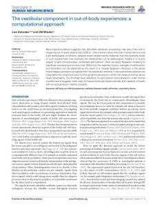
Figure 1. Plot of the calculated magnetic field magnitudes for Venus.
Figure 3, Plot of the calculated Mach number values and plasma streamlines in the equatorial plane for the comet. The figure shows an approximately 2 x 3 Mkm region.
Figure 2. Plot of the measured x component of the magnetic field during Pioneer Venus orbit 1642 and the corresponding calculated values (smooth curve) for Venus,
Figure 4. Plot of the calculated magnetic field magnitude and magnetic field lines in the equatorial plane for the comet. The figure shows an approximately 2 x 3 Mkm region.
520
Figure 5. Plot of the calculated Mach n u m b e r values and plasma streamlines in the equatorial plane for the comet. The figure shows an approximately 50,000 x 30,000 km region.
,
.
,
i
,
•
.
i
.
•
Figure 6. Plot of the calculated magnetic field magnitude and magnetic field lines in the equatorial plane for the comet. The figure shows an approximately 50,000 x 30,000 km region.
T
lOs £ ,~
I0 --
Olu model Giotto M a g n e ~ , e ~
1os Giotto I M S - H E R S W e g m a n n et al. 1 9 8 7
---
~'.~ ' ~ . ~ ' ; _ ~ . C o m e t o c e n t r i c
l
.
,
I
,
.
z,~oa Distance
.
i
. ,
~-JO 6-10
[krnl
Figure 7. Comparison of the m o d e l e d magnetic field magnitude with the measured magnetic field along the Giotto trajectory for the comet.
ioz
i
i
I
i
l i l i [
,. i
i
f
~o4
io3 C o m e t o c e n t r i c
D i s t a n c e
. . . .
•
tos {kml
Figure 8. Comparison of the m o d e l e d plasma densi~" with measured ion mass density along the Giotto i n b o u n d pass as a function of cometocentric distance for the comet.
521
where lk and rk are the left and right eigenvectors associated with the k th wave. The decision of which formula to use is made based on economy: if there are more right-going waves than left-going waves, the first formula is used; if the converse is true, the second formula is used. Results Results are shown for two cases. (These cases are discussed more fully elsewhere [5, 6].) The first case, shown in Figures 1 and 2, is an axisymmetric calculation of the interaction of the solar wind with Venus under conditions where the interplanetary field is approximately aligned with the solar-wind velocity. In Figure 1, contours of the magnitude of the magnetic field are shown, with the bow shock, tail shock and tail magnetosheath in evidence. Figure 2 shows a comparison of the calculated axial component of magnetic field with data from the Pioneer Venus Orbiter (taken from a time that the interplanetary field was only 7.6" from the nominal solar-wind direction). Qualitatively, the agreement is fair, although the magnitude of the magnetic-field reveral is underestimated. The second case, shown in Figures 3-8, is a three-dimensional calculation of the interaction of the solar wind with the comet P/Halley. The Mach number and magnetic field far from the comet are shown in Figures 3 and 4, with the bow shock in evidence at about 350,000 krn upstream of the comet. Figures 5 and 6 show a blow-up of the near-comet region (the scale is approximately 1/50th that of Figures 1 and 2), with contact surface and inner shock in evidence. Figures 7 and 8 show comparisons of the computed magnetic field and density with data from the Giotto spacecraft. As space physics data go, the comparison is remarkably good.
References [1] K. G. Powell, "Solution of the euler and magnetohydrodynamics equations on solutionadaptive cartesian grids," in Computational Fluid Dynamics, Von K£rmhn Institute for Fluid Dynamics, Lecture Series 1996-06, 1996. [2] K. G. Powell, P. L. Roe, R. S. Myong, T. I. Gombosi, and D. L. DeZeeuw, "An upwind scheme for magnetohydrodynamics," in AIAA 12th Computational Fluid Dynamics Conference, 1995. [31 P. L. Roe and D. S. Balsara, "Notes on the eigensystem of magnetohydrodynamics," SIAM Journal of Applied Mathematics, vol. 56, no. 1, 1996. [4] G. Gallice, "Resolution numerique des equations de la magnetohydrodynamique ideale bidimmensionale," in Mdthodes numdriques pour la MHD, 1995. [5] T. I. Gombosi, D. L. D. Zeeuw,R. M. Hgberli, and K. G. Powell, "A 3D multiscale MHD model of cometary plasma environments," Journal of Geophysical Research, vol. 101, 1996. [6] D. L. D. Zeeuw, T. I. Gombosi, A. Nag'y, K. G. Powell, and J. Luhman, "A new axisymmetric MHD model of the interaction of the solar wind with venus," Journal of Geophysical Research, vol. 101, 1996.