A Computational Fluid Dynamics Study of Transitional Flows in Low ...

Y. B. Suzen Assistant Professor Department of Mechanical Engineering and Applied Mechanics, North Dakota State University, Fargo, ND 58105

P. G. Huang Professor and Chair Mechanical and Materials Engineering Department, Wright State University, Dayton, OH 45435

D. E. Ashpis Aerospace Engineer Mem. ASME NASA Glenn Research Center at Lewis Field, Cleveland, OH 44135

R. J. Volino Associate Professor Mem. ASME Department of Mechanical Engineering, United States Naval Academy, Annapolis, MD 21402-5042

T. C. Corke Clark Chair Professor Fellow ASME

F. O. Thomas Professor Mem. ASME

J. Huang Graduate Assistant Department of Aerospace and Mechanical Engineering, Center for Flow Physics and Control, University of Notre Dame, Notre Dame, IN 46556

A Computational Fluid Dynamics Study of Transitional Flows in Low-Pressure Turbines Under a Wide Range of Operating Conditions A transport equation for the intermittency factor is employed to predict the transitional flows in low-pressure turbines. The intermittent behavior of the transitional flows is taken into account and incorporated into computations by modifying the eddy viscosity, ^t, with the intermittency factor, y. Turbulent quantities are predicted by using Menter’s twoequation turbulence model (SST). The intermittency factor is obtained from a transport equation model which can produce both the experimentally observed streamwise variation of intermittency and a realistic profile in the cross stream direction. The model had been previously validated against low-pressure turbine experiments with success. In this paper, the model is applied to predictions of three sets of recent low-pressure turbine experiments on the Pack B blade to further validate its predicting capabilities under various flow conditions. Comparisons of computational results with experimental data are provided. Overall, good agreement between the experimental data and computational results is obtained. The new model has been shown to have the capability of accurately predicting transitional flows under a wide range of low-pressure turbine conditions.

[DOI: 10.1115/1.2218888]

J. P. Lake Special Projects Flight Commander, 586th FLTS/DON, Holloman AFB, NM 88330

P. I. King Professor Mem. ASME Department of Aeronautics and Astronautics, Air Force Institute of Technology, Wright-Patterson AFB, OH 45433

1 Introduction

The process of transition from laminar to turbulent flow is a major unsolved problem in fluid dynamics and aerodynamics. One Contributed by the Turbomachinery Division of ASME for publication in the J OURNAL OF TURBOMACHINERY. Manuscript received February 14, 2004; final manuscript received February 13, 2006. Review conducted by R. L. Davis.

area where the transition process plays an important role and is even more complicated due to the diverse flow conditions encountered is the low-pressure turbine applications. Transitional flows in these applications are affected by several factors such as varying pressure gradients, wide range of Reynolds number and freestream turbulence variations, flow separation, and unsteady wake-boundary layer interactions. Accurate simulation and prediction of transitional flows under these diverse conditions is key

Journal of Turbomachinery Copyright © 2007 by AIAA. Reprinted by permission.

JULY 2007, Vol. 129 / 527

Downloaded 10 Dec 2008 to 128.156.10.80. Redistribution subject to ASME license or copyright; see http://www.asme.org/terms/Terms_Use.cfm

to design of more efficient jet engines. In low-pressure turbine applications, flow over the blades is mostly turbulent at the high Reynolds number conditions encountered at takeoff and the efficiency is at its design maximum. However, at lower Reynolds number conditions which correspond to high altitudes and cruise speeds the boundary layers on the airfoil surface have a tendency to remain laminar; hence, the flow may separate on the suction surface of the turbine blades before it becomes turbulent. This laminar separation causes unpredicted losses, substantial drops in efficiency, and increase in fuel consumption [ 1–3 ] . In order to calculate the losses and heat transfer on various components of gas turbine engines, and to be able to improve component efficiencies and reduce losses through better designs, accurate prediction of development of transitional boundary layers is essential [ 1 ]. One approach proven to be successful for modeling transitional flows is to incorporate the concept of intermittency into computations. This can be done by multiplying the eddy viscosity obtained from a turbulence model, /.at, used in the diffusive parts of the mean flow equations, by the intermittency factor, y ( Simon and Stephens [4 ]). This method can be easily incorporated into any Reynolds averaged Navier-Stokes solver. In this approach, the intermittency factor, y, can be obtained from an empirical relation such as the correlation of Dhawan and Narasimha [ 5 ], or it can be obtained from a transport model. Dhawan and Narasimha [5] correlated the experimental data and proposed a generalized intermittency distribution function across flow transition. Gostelow et al. [ 6] extended this correlation to flows with pressure gradients under the effects of a range of freestream turbulence intensities. Solomon et al. [7 ], following the work of Chen and Thyson [ 8 ], developed an improved method to predict transitional flows involving changes in pressure gradients. These empirical methods led to development of transport equations for intermittency. Steelant and Dick [9] proposed a transport equation for intermittency, in which the source term of the equation is developed such that the y distribution of Dhawan and Narasimha [ 5] across the transition region can be reproduced. Steelant and Dick used their model, coupled with two sets of conditioned Navier-Stokes equations, to predict transitional flows with zero, favorable, and adverse pressure gradients. However, since their technique involved the solution of two sets of strongly coupled equations, the method is not compatible with existing computational fluid dynamics (CFD) codes, in which only one set of Navier-Stokes equations is involved. Moreover, the model was designed to provide a realistic streamwise y behavior but with no consideration of the variation of y in the cross-stream direction. Cho and Chung [ 10] developed a k- e - y turbulence model for free shear flows. Their turbulence model explicitly incorporates the intermittency effect into the conventional k- e model equations by introducing an additional transport equation for y. They applied this model to compute a plane jet, a round jet, a plane far wake, and a plane mixing layer with good agreement. Although this method was not designed to reproduce flow transition, it provided a realistic profile of y in the cross-stream direction. Suzen and Huang [ 11] developed an intermittency transport equation combining the best properties of Steelant and Dick’s model and Cho and Chung’s model. The model reproduces the streamwise intermittency distribution of Dhawan and Narasimha [ 5] and also produces a realistic variation of intermittency in the cross-stream direction. This model has been validated against European Research Community On Flow Turbulence And Combustion (ERCOFTAC) benchmark T3-series experiments reported by Savill [ 12,13 ] , low-pressure turbine experiments of Simon et al. [ 14 ] , and separated and transitional boundary layer experiments of Hultgren and Volino [ 15] with success [ 11,16–21 ] . In this paper we concentrate on prediction of three recent lowpressure turbine experiments on the Pratt and Whitney’s Pack B 528 / Vol. 129, JULY 2007

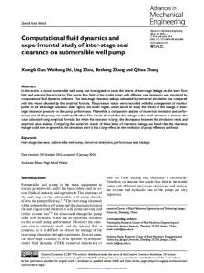
Fig. 1 P&W Pack B blade cascade details

blade under low Reynolds number conditions using the transport model for intermittency. Due to the fact that the Pack B blade is very sensitive to changes of flow conditions, it is an ideal test blade for validating the transition/turbulence models. The three sets of experiments considered are conducted by Lake et al. [ 3,22 ] , Huang et al. [ 23 ] , and Volino [ 24] at three independent facilities. These experiments provide an extensive database for investigating transitional flows under low-pressure turbine conditions and are employed as benchmark cases for further testing of the predicting capabilities of the current intermittency model. A summary of the experiments are given in the next section. In Sec. 3, the intermittency transport model is presented and implementation of the model and the empirical correlations employed for the onset of transition are described. In Sec. 4, the predictions of the new intermittency model are compared against the experimental data. Conclusions are provided in Sec. 5. 2 Low-Pressure Turbine Experiments

In this paper, we concentrate on computation of three sets of low-pressure turbine experiments using the intermittency transport model. These experiments are conducted by Lake et al. [3,22 ] , Huang et al. [ 23 ] , and Volino [24 ] . In these experiments Pratt and Whitney’s Pack B blade is used; the details of the blade are shown in Fig. 1. Overall, these experiments cover a Reynolds number range from 10,000 to 172,000 and the freestream turbulence intensity ranges from 0.08% to 4%. The cases and data used for comparison in this paper are summarized in Table 1. In the following sections details of these experimental efforts are given. 2.1 Pack B Blade Cascade Experiments of Lake et al. [3,22]. Lake et al. [ 3,22] conducted experiments on the Pack B blade in order to identify methods for reducing separation losses on low-pressure turbine blades under low Reynolds number conditions. In the experiments, they investigated flows at low Reynolds numbers of 43,000, 86,000, and 172,000 based on inlet Transactions of the ASME


Table 1 Details of the experiments used for comparison with computations Cx

Re

Source

Test Section

(m)

(Uin Cx / ^)

FSTI (%)

Lake et al. [3,22]

P&W Pack B cascade

0.1778

86,000 172,000 10,000 25,000 50,000

1&4 1&4 0.08 0.08 0.08, 1.6, 2.85

75,000

0.08, 1.6, 2.85

100,000

0.08, 1.6, 2.85

10,291

0.5

20,581

0.5

41,162

0.5

82,324

0.5

Huang et al. [23]

Volino [24]

P&W Pack B cascade

P&W Pack B single passage

0.1595

0.1537

Data used for Comparison distribution distribution Cp distribution Cp distribution Cp distribution, velocity profiles a Cp distribution, velocity profiles a C distribution, velocity profilesa Cp distribution, velocity profiles Cp distribution, velocity profiles Cp distribution, velocity profiles Cp distribution, velocity profiles Cp Cp

aVelocity profiles are available for FSTI=0.08% and 2.85% from experiments

velocity and axial chord and freestream turbulence intensities (FSTI) of 1% and 4%. These conditions are similar to those encountered at high-altitude, low-speed flight of reconnaissance unmanned aerial vehicles used by USAF. In Lake’s experiments, surface pressure coefficients, boundary layer velocity, and turbulence profiles, total pressure loss data were obtained at FSTI=1% and FSTI=4%. The test setup shown in Fig. 2 included eight blades with axial chord of 0.1778 m

( 7 in. ) , and blade spacing of 0.1575 m ( 6.2 in. ) . The blades were numbered 1 through 8 starting from the inside bend. Boundary layer measurements were taken on blade 5 and surface pressures were measured around blades 4 and 6. In this paper, the Pack B blade experiments with Reynolds numbers of 86,000 and 172,000 and freestream turbulence intensities of 1% and 4% are computed and comparison of pressure distributions between experiments and computations are performed.

Fig. 2 Experimental setup used by Lake et al. [3,22] Journal of Turbomachinery

JULY 2007, Vol. 129 / 529


Fig. 3 Comparison of computed and experimental decay of turbulence for experiments of Huang et al. [23], with grid 0

2.2 Pack B Blade Cascade Experiments of Huang et al. [23]. Huang et al. [23] conducted experiments on Pack B blade cascade for a range of Reynolds numbers and turbulence intensities. The Reynolds numbers range from 10,000 to 100,000 based on inlet velocity and axial chord as listed in Table 1. In their experiments the blades had an axial chord length of 0.1595 m ( 6.28 in. ) . The freestream turbulence intensity in the tunnel was measured as 0.08%. In order to increase the turbulence intensity, two grids with different mesh sizes were used. One of the grids had the mesh size of 0.0254 m (denoted as grid 0) and the other had 0.008 m (denoted as grid 3 ) . The decay of turbulence after the grids was measured using crosswire and they are shown in Figs. 3 and 4 along with the computed results for grid 0 and grid 3, respectively. The grids were movable in the tunnel so that the turbulence level of the flow that reaches the blades could be controlled by moving the grid that is, by increasing or decreasing the distance between the grid and the blade. Experiments were performed for Reynolds numbers 50,000, 75,000, and 100,000, with grids placed 0.762 m ( 30 in.) away from the blade leading edge, corresponding to turbulence intensities of 2.85% and 1.6% at the leading edge for grid 0 and grid 3, respectively. For Re =100,000, grid 0 is placed at 0.5588 m ( 22 in.) and 0.3556 m ( 14 in. ) , corresponding to turbulence intensities of 3.62% and 5.2%, respectively. Pressure coefficient data are available for all cases and detailed boundary layer measurements are available for Re=50,000, 75,000, and 100,000 with FSTI=0.08% and 2.85% cases. The cases and data used for comparisons in this paper are listed in Table 1.

Fig. 5 Schematic of the test section for experiments of Volino [24]

2.3 Pack B Experiments of Volino [24]. Volino [ 24] investigated the boundary layer separation, transition, and reattachment under low-pressure turbine airfoil conditions. The experiments included five different Reynolds numbers ranging between 10,291 and 123,492 and freestream turbulence intensities of 0.5% and 9%. The test section consisted of a single passage between two Pack B blades as shown in Fig. 5. The axial chord length of the blades was 0.1537 m ( 6.05 in. ) . There are flaps located upstream of each blade to control the amount of bleed air allowed to escape from the passage. These flaps were adjusted by matching measured pressure distribution for a high Reynolds number with the inviscid pressure distribution on the blade. In addition to the upstream bleed flaps, a tailboard on the pressure side was used to set the pressure gradient. The compiled data include pressure surveys, mean and fluctuating velocity profiles, intermittency profiles, and turbulent shear stress profiles. It was observed that the effect of high Reynolds number or high freestream turbulence level was to move transition upstream. Transition started in the shear layer over the separation bubble and led to rapid boundary layer reattachment. At the lowest Re case, transition did not take place before the trailing edge and the boundary layer did not reattach. The beginning of transition corresponded to the beginning of a significant rise in the turbulent shear stress. These experimental results provide detailed documentation of the boundary layer and extend the existing database to lower Reynolds numbers. The cases used for comparisons with computations in this paper are listed in Table 1 along with the type of data used for comparisons.

3 Intermittency Transport Model

Fig. 4 Comparison of computed and experimental decay of turbulence for experiments of Huang et al. [23], with grid 3

530 / Vol. 129, JULY 2007

In this section, the transport model for intermittency is presented. The model combines the transport equation models of Steelant and Dick [ 9] and Cho and Chung [ 10 ] . Details of the development and implementation of the transport model are given in Suzen and Huang [ 11,16,17 ] , and in Suzen et al. [ 18 ] . The model equation is given by Transactions of the ASME


dpy dt

+

dpuiy dxj ( 1 − F) 2 C0 p uu kf (s)f' (s)

= ( 1 − y) + + C3 p

C1y du i Tij— k dxj

F

k 3/2 ui dui dy 1/2 k u k) dxj dxj

− C2yp— e (u

k2 dy dy e dxj dxj

+a x (( ( 1− y)yory /i + ( 1− y)ory / l

t J,

j

The distributed breakdown function, as' 4

f(s)

+ bs' 3

( 1)

) dy ) dxj

has the form

2

+ cs' + ds' + e ( 2) + h where s' = s − s t, and s is the distance along the streamline coordinate, and st is the transition location. The coefficients are f(s) =

a

c =0.204(

gs' 3

nor

=50

no r −0.5 U

U

b =−0.4906

d =0.0 e

h =10 e The shear stresses are defined as

g

=0.04444(

=50

no r U

−1.5

( 3)

M [1−exp(0.75X10

nôr

2 duk 2 T = /..6: − - & − - pk Sij (4) + dxj dx i 3 dx 3 The blending function F is constructed using a nondimensional parameter k/ Wv, where k is the turbulent kinetic energy and W is the magnitude of the vorticity. The blending function has the form j

ij

k

k/ Wv 200(1− y0.1)0.3 The model constants used in Eq. ( 1) are F

( 7) 1.8 X 10 −11 Tu7/4 When flows are subject to pressure gradients, the following correlation is used nô r = (nv 2/ U3 )o r=

)

du i du '

ij

processors are used during the computations, it is more efficient to divide the computational domain into several smaller pieces with very fine grids and distribute the zones to processors with the consideration of load balancing. This code has been used extensively in a recent turbulence model validation effort (Hsu et al. [ 26]) and computations of unsteady wake/blade interaction ( Suzen and Huang [27]) conducted at the University of Kentucky. The multiblock grid systems used in the computations are obtained by conducting a series of grid refinement studies in order to ensure that the details of the flow field are captured accurately and the results are grid independent. All grid systems have first y+ less than 0.5 near solid walls. In using this intermittency approach, the turbulence model selected to obtain /it must produce fully turbulent features before transition location in order to allow the intermittency to have full control of the transitional behavior. Menter’s [ 28] SST model satisfies this requirement. It produces almost fully turbulent flow in the leading edge of the boundary layer and therefore is used as a baseline model to compute /it and other turbulent quantities in the computations [ 18 ] . The value of nor used in evaluating the constants given by Eq. ( 3) is provided by the following correlation for zero-pressure gradient flows [ 18]

(

__ tanh 4

oryl = oryt =1.0 C0 =1.0 C 1

5)

= 1.6

(nôr) ZPG

10− 3227Kt

0.5985

,

6

Kt Tu

−

0.7)]

Kt >

Kt
0 ) is from Steelant and Dick [9 ]. The portion of the correlation for adverse pressure gradient flows for Kt < 0 is formulated using the transition data of Gostelow et al. [6] and Simon et al. [ 14] ( Suzen et al. [ 18] ) .

C2 =0.16 C 3

=0.15 The intermittency is incorporated into the computations simply by multiplying the eddy viscosity obtained from a turbulence model, /it, by the intermittency factor, y. Simon and Stephens [4] showed that, by combining the two sets of conditioned Navier-Stokes equations and making the assumption that the Reynolds stresses in the nonturbulent part are negligible, the intermittency can be incorporated into the computations by using the eddy viscosity, i which is obtained by multiplying the eddy viscosity from a turbulence model, /it, with the intermittency factor, y. That is

/ tJ

*

/it

( 6) = y/it is used in the mean flow equations. It must be noted that y does not appear in the generation term of the turbulent kinetic energy equations. Computations of the experiments are performed using a recently developed multiblock Navier-Stokes solver, called GHOST. The code was developed at the University of Kentucky, by Huang, and is a pressure-based code based on the SIMPLE algorithm with second-order accuracy in both time and space. Advection terms are approximated by a QUICK scheme and central differencing is used for the viscous terms. The “Rhie and Chow” momentum interpolation method [ 25] is employed to avoid checkerboard oscillations usually associated with the nonstaggered grid arrangement. This code is capable of handling complex geometries, moving, and overset grids and includes multiprocessor computation capability using message passing interface (MPI ) . Since multiple Journal of Turbomachinery

Fig. 6 Multiblock grid used for computations of experiments of Lake et al. [3,22] and FSTI=0.08% experiments of Huang et al. [23] JULY 2007, Vol. 129 / 531


Fig. 7 Comparison of computed pressure coefficient with experiments of Lake et al. [3,22]

The current approach uses the intermittency transport model to obtain the intermittency distribution for the transitional flows, while the onset of transition is defined by correlations. The onset of attached flow transition is determined by the following correlation in terms of turbulence intensity, Tu, and the acceleration parameter, Kt , Re ot = ( 120 + 150 Tu — 2/3 ) coth [4 ( 0.3 — Kt X

( 9) 105 )] where Kt was chosen as the maximum absolute value of that parameter in the downstream deceleration region [ 18 ] . This correlation maintains the good features of Abu-Ghannam and Shaw [ 29] correlation in the adverse pressure gradient region, and in addition reflects the fact that the flow becomes less likely to have transition when subject to favorable pressure gradients by rapidly rising as Kt becomes positive. In order to determine the onset of separated flow transition Re st is expressed in terms of the turbulence intensity (Tu) and the momentum thickness Reynolds number at the point of separation (Reos ) in the form [ 19]

Rest = 874ReBs 1 exp [ — 0.4 Tu ] ( 10) This correlation provides a better representation of the experimental data than Davis et al. [30] correlation and is used to predict onset of separated flow transition in the present computations. 532 / Vol. 129, JULY 2007

4 Results and Discussion 4.1 Simulations of Experiments of Lake et al. [3,22]. The intermittency model is applied to predict the Pack B blade experiments of Lake et al. [3,22 ] . In the computations, flows at Reynolds numbers of 86,000 and 172,000 based on inlet velocity and axial chord with freestream intensities of 1% and 4% were investigated. The computations were performed using the grid system shown in Fig. 6 consisting of five zones obtained as a result of a grid refinement study. In the grid refinement study computations were performed on a series of successively finer grids and the variations in the results were observed. The grid shown in Fig. 6 was chosen to be adequate for obtaining grid-independent solutions for all cases. The four zones on which the blade grid is superposed each have 125 X 225 grid points and the O-type grid around the blade has 401 X 101 points with first y+ less than 0.5. The comparisons of computed and experimental pressure coefficient distributions are shown in Figs. 7 (a)– 7 (d). In these figures, the experimental distributions correspond to the measurements made on test blades 4 and 6. The computed results compare well with the experiments for high turbulence intensity, FSTI=4%, cases shown in Figs. 7 (a ) and 7 (c). However, for FSTI=1% cases shown in Figs. 7 (b) and Transactions of the ASME


Fig. 8 Comparison of computed total pressure loss coefficients with experiments of Lake et al. [3,22] and Huang et al. [23]

7 (d), the extent of the separation bubbles is underpredicted in the computations. For example, for Re=86,000, FSTI=1%, shown in Fig. 7 (d), the flow reattaches earlier in computations than it does in the experiment, as can be observed from the difference in the pressure coefficient distributions between x/C x =80 to 85%. The comparison of computed total pressure loss coefficients with experiments is shown in Fig. 8. For the Re=86,000 case, the computed loss coefficient is in good agreement with the experiments for both FSTI levels. However, for the Re=172,000 case the computations underpredicted the loss coefficient compared to experiments for both FSTI=1% and FSTI=4%. From Fig. 8 it is evident that the cascade losses decrease as the Reynolds number increases. This reduction in cascade losses with increasing Reynolds number is due to the decrease in size of the separated flow region on the suction side of the blades. The onset of separation locations, reattachment locations, and onset of transition locations on the suction surface are summarized in Table 2 for these cases, along with the corresponding values from experiments. In the experiments, the onset of transition locations and the reattachment locations are not reported. The experimental onset of separation and reattachment points are extracted from the experimental pressure coefficient data. The onset of separation is taken to be the axial location where the plateau in the pressure coefficient distribution of the suction side begins, and the reattachment point is taken to be the axial location after the sharp change in Cv following the plateau. This procedure may lead to an error of approximately ±1.5% of axial chord in the estimated onset locations. The onset of separation, reattachment, and onset of transition locations are plotted against Reynolds number in Figs. 9 (a) and 9 (b) for FSTI=4% and 1%, respectively. The uncertainty in the estimated experimental values is indicated by error bars in the figures. For the high turbulence intensity case, computation predicts onset of separation and reattachment slightly upstream of the experiment. For the low FSTI case shown in Fig. 9 (b), the separation zone is predicted smaller than the experiments. The onset of transition is predicted over the separated flow region in the shear

Fig. 9 Comparison of separation, reattachment, and transition locations for experiments of Lake et al. [3,22]

layer. From comparison of these figures it is evident that, with decreasing freestream turbulence intensity, the separation zone becomes larger, and for a given FSTI condition, the separated flow region gets smaller with increasing Reynolds number. 4.2 Simulations of Experiments of Huang et al. [23]. In this set of experiments, first the cases with no grid in tunnel corresponding to FSTI=0.08% are computed. In these computations, the same grid system used for the computations of experiments of Lake et al. [3,22] shown in Fig. 6 is used. The comparisons of the computed and the experimental pressure coefficients are shown in Figs. 10 (a)–10 (e) for Re=100,000, 75,000, 50,000, 25,000, and 10,000 based on inlet velocity and axial chord. The agreement between the experiments and computations is very good for all cases. The computed total pressure loss coefficients are compared to the available data for Re=25,000 and 50,000 in Fig. 8. The loss coefficients predicted in the computations are 2% to 3% higher compared to the experiments for both Reynolds numbers. The onset of separation, transition, and reattachment locations are tabulated in Table 3 for all cases and plotted against Reynolds number in Figs. 11 (a) –11 (c) for FSTI=0.08%, 1.6%, and 2.85%,

Table 2 Separation, reattachment, and transition locations for cases of Lake et al. [3,22] Re ( Uin Cx / ^)

FSTI (%)

xs / Cx (Computation)

xs / Cx (Experiment)

xr / Cx (Computation)

xr / Cx (Experiment)

xtr / Cx (Computation)

172,000 86,000 172,000 86,000

4 4 1 1

0.732 0.725 0.728 0.722

0.74 0.74 0.72 0.72

0.83 0.86 0.82 0.87

0.84 0.88 0.84 0.90

0.806 0.832 0.808 0.849

Journal of Turbomachinery

JULY 2007, Vol. 129 / 533


x / C, (%)

x / C, (%)

Fig. 10 Comparison of computed pressure coefficients with experiments of Huang et al. [23] for FSTI=0.08% cases

respectively. Computed velocity profiles at seven axial stations along the suction surface of the blade are compared to the experiments for Re=100,000, 75,000, and 50,000 in Figs. 12–14, respectively. For the Re=100,000 case, the computed velocity profiles compare very well with the experiment as shown in Figs. 12 (a)–12 (g) . At the first three measurement stations, flow is laminar and attached as shown in Figs. 12 (a) –12 (c) . Flow separation takes place at x/ Cx =0.725 and the separated flow region is visible in Figs. 12 (d) and 12 ( e) , corresponding to axial locations of x/ Cx =0.75 and 0.80. The flow transition and reattachment takes place around x/ Cx =0.84 in the computation. Reattachment location is earlier than the experiment which takes place at x/ C x =0.875. In Fig. 12 (f) corresponding to axial station of x/ Cx =0.85 the computed flow field has already attached, although the experimental profile indicates a very small separation zone close to wall. At x/ Cx =0.9 the flow is completely attached as shown in Fig. 12 (g ) . When the Reynolds number is reduced to 75,000, the size of the separation bubble increases as can be observed from the comparison of the velocity profiles shown in Figs. 13 (a)–13 (g ) . At this Reynolds number the flow separates around x/ Cx ~ 0.72 and reattaches around x/ Cx ~ 0.87. The transition onset location is pre-

dicted at x/ Cx =0.854. The size of the separation bubble is larger than the Re=100,000 case from comparison of Figs. 13 (d)–13 (f) and 12 (d)–12 (f) . Next, the Reynolds number is reduced to 50,000 and the comparison of computed and experimental velocity profiles is shown in Figs. 14 (a) –14 (g ) . For this case the separation bubble is much larger from the previous cases and extends until x/ Cx ~ 0.975 in the experiment and x/ Cx ~ 0.93 in the computations, as can be seen in Figs. 14 (d)–14 (g) . Computations predicted the transition onset location at x/ Cx =0.89. In the computations, the onset of separation is predicted well in agreement with experiment; however, the reattachment point is earlier, making the size of the separation bubble smaller when compared to experiment. This is evident from the comparison of velocity profiles at the last two stations shown in Figs. 14 (f) and 14 (g) . The onset of separation and reattachment points for FSTI =0.08% cases is predicted upstream of the experiments as shown in Fig. 11 (a ) . Next, the high FSTI cases are computed using the six zone multiblock grid system shown in Fig. 15. The computational domain is extended upstream of the blade in order to specify the correct turbulence intensity at the inlet and to match the decay of

Table 3 Separation, reattachment, and transition locations for cases of Huang et al. [23] Re ( Uin Cx / ^)

FSTI (%)






10,000 25,000 50,000 75,000 100,000 50,000 75,000 100,000 50,000 75,000 100,000

0.08 0.08 0.08 0.08 0.08 1.6 1.6 1.6 2.85 2.85 2.85

0.661 0.656 0.714 0.718 0.725 0.722 0.728 0.732 0.728 0.732 0.735

0.725 0.725 0.725 0.725 0.725 0.728 0.730 0.730 0.722 0.729 0.734

0.980 0.925 0.860 0.840 0.900 0.867 0.860 0.887 0.840 0.842

0.975 0.870 0.875 0.900 0.875 0.877 0.900 0.870 0.850

0.936 0.890 0.854 0.840 0.854 0.834 0.821 0.837 0.816 0.806

534 / Vol. 129, JULY 2007

Transactions of the ASME


The computed size and extent of the separation bubble is in good agreement with the experiment as tabulated in Table 3 and as can be seen in Figs. 11 (c ) and 16 (lc)–16 (f) . For the lower Reynolds number of 75,000, computed velocity profiles are compared with the experiments in Figs. 18 (a) –18 (g) . The agreement between experiment and computation is good prior to the reattachment as shown in Figs. 18 (a)–18 (e) . There is a discrepancy in the reattachment region. The flow separation takes place around x / Cx ~ 0.73 and reattaches at x / Cx ~ 0.87 according to the experiment, whereas computation predicts reattachment earlier at around x / Cx ~ 0.84 with the onset of transition predicted at x / Cx =0.816. The difference in reattachment points is evident in the comparison of the computed and experimental velocity profiles shown in Fig. 18 (f) . At this station the experimental profile indicates separated flow and the computed profile shows an already attached flow. The next case considered has the same FSTI=2.85%o but with Reynolds number being reduced to 50,000. The comparison of velocity profiles is shown in Figs. 19 (a )–19 (g) . The computations agree well with the experiment, and the size and extent of the separation bubble are well predicted as can be seen from Fig. 11 ( c) . The onset of separation is around x / Cx ~ 0.72 and the flow reattaches around x / Cx ~ 0.9, with transition onset at x / Cx =0.837. In Fig. 20, computed and experimental pressure coefficient distributions for grid 3 case which correspond to FSTI=1.6%o are compared for Re=50,000, 75,000, and 100,000. Again, very good agreement between computations and experiments is obtained. The onset of separation and reattachment locations shown in Fig. 11 (b ) compares well with the experiments. Overall, Figs. 11 (a) –11 (c) indicate that, as FSTI increases, the separated flow region decreases, and at a given FSTI, increasing Reynolds number has the same effect on the separated flow region.

Fig. 11 Comparison of separation, reattachment, and transition locations for experiments of Huang et al. [23]

turbulence that reaches the blade. The matched computed and experimental turbulence decays are shown in Figs. 3 and 4 for grid 0 and grid 3, respectively. The cases considered have the grids placed 0.762 m ( 30 in) upstream of the blade, corresponding to turbulence intensities of 2.85%o and 1.6%o for grid 0 and grid 3, respectively. The comparison of the computed and the experimental pressure coefficient distributions for Re=50,000, 75,000, and 100,000 for FSTI=2.85%o cases is shown in Fig. 16. The agreement is very good between computations and experiments. Comparisons of computed velocity profiles with the experiments for Re=100,000 are given in Figs. 17 (a) –17 (g) . In this case, the flow separates around x / Cx ~ 0.74 and reattaches at x / Cx ~ 0.85. The onset of transition is predicted at x / Cx =0.806. Journal of Turbomachinery

4.3 Simulations of Pack B Experiments of Volino [24]. In computation of experiments of Volino [ 24] the flow field is modeled with the 31-zone multiblock grid shown in Fig. 21 obtained as a result of a series of grid refinement studies. The bleed flaps below the lower blade and above the upper blade are defined by fitting third-order polynomials through the available points obtained from experimental setup; these curves are used as the flap shapes in generating the computational grid. Initial computations indicated that the shape of the bleed flaps and the orientation of the tailboard behind the upper blade greatly affect the computed results, especially the onset of separation and reattachment points on the lower blade’s suction surface. In order to select the most accurate orientation for the tailboard and the shape of the bleed flaps, several test computations were performed for the case with Re=41,162 and FSTI=0.5%o using different tailboard orientations and bleed flap shapes. In these computations the main goal was to match the experimental velocity profiles in the laminar flow part and to capture the correct onset point of separation. Once an acceptable geometry is obtained, the final bleed flap shapes and tailboard orientation are used for computation of all other Reynolds number cases. Computed pressure coefficient distributions are compared to experiments in Figs. 22 (a)–22 (lc) for Re=82,324, 41,162, 20,581, and 10,291, and the separation onset, reattachment, and transition onset information is summarized in Table 4. The Cp comparison for Re= 82, 324 shown in Fig. 22 (a) indicates that the computation predicts early reattachment of the flow; in the recovery region following reattachment the pressure coefficient distribution is overpredicted. The computed pressure coefficient distributions for the lower Reynolds number cases shown in Figs. 22 (c ) and 22 (cl) compare well with experiments. For the Re=41,162 case shown in Fig. 22 (b ) , the onset of separation and reattachment locations matches the experiment as given in Table 4; however, in the recovery reJULY 2007, Vol. 129 / 535


Fig. 12 Comparison of computed velocity profiles with experiments of Huang et al. [23], Re=100,000, FSTI=0.08% case



Fig. 15 Grid used for computation of experiments of Huang et al. [23] with FSTI=1.6% and 2.85%

536 / Vol. 129, JULY 2007

gion the pressure coefficient distribution is overpredicted. Computed velocity profiles are compared to experiment at 11 stations along the suction surface of the blade in Figs. 23 (a)–23(k) for Re=82,324 and FSTI=0.5%. The results compare well with the experiment up to x/Cx=0.732 shown in Figs. 23 (a)–23(g). After this station flow separation takes place. Separation onset and reattachment are slightly earlier in the computations compared to experiment as given in Table 4. This also can be observed from the velocity profiles at stations x/Cx=0.798 to 0.912 shown in Figs. 23(h)–23 (j ). Overall computations compare well with the experimental measurements. Next the Reynolds number is reduced to 41,162 and the computed and experimental velocity profiles are compared in Figs. 24(a)–24(k). The computed profiles agree well with experiments except at x/ Cx =0.912 shown in Fig. 24 (j). At this station the computation indicates a smaller separated flow region close to reattachment in contrast to the experiment. However, the flow reattaches around x/ Cx =0.95 both in computation and experiment, and in the next measurement station the agreement is well. The next case considered has a Reynolds number of 20,581. Computed velocity profiles are shown along with the experimental data at 11 axial stations in Figs. 25 (a)–25(k). In this case flow separates around x/ Cx ~ 0.76 and does not reattach in experiment; however, computations indicated reattachment at x/ Cx ~ 0.98. This discrepancy is evident from the comparison of velocity proTransactions of the ASME


X

/ C, (%)

X / C,

(%)

X/C. (%)

Fig. 16 Comparison of computed pressure coefficients with experiments of Huang et al. [23] for FSTI=2.85% cases 0.1 . U

T

(a)

(b)

(e)

(d)

(e)

f

(g)

x/Cx =0.5

x /Cx =0.6

x /Cx=0.7

xtCx=0.75

x/Cx=0.80

X C x 0.8E

x/Cx=0.9

Computa5on Experiment

0.05

0

0

1 U/U„

2

0

1 U/U„

2

0

1 UIU,,,

2

0

1 U/U,,,

2

0

1 U/U,,,

2

0

1 U/U,,,

2

0

1 U/U„

2

Fig. 17 Comparison of computed velocity profiles with experiments of Huang et al. [23], Re=100,000, FSTI=2.85% case 0.1 . U

T

(a)

(b)

(e)

(d)

(e)

f

(g)

x/Cx =0.5

x /Cx =0.6

x /Cx=0.7

xJCx=0.75

x/Cx=0.80

X C x 0.85

x/Cx=0.9


0.05

0

0

1 U/U„

2

0

1 U/U„

2

0

1 UIU,,,

2

0

1 U/U,,,

2

0

1 U/U,,,

2

0

1 U/U,,,

2

0

1 U/U„

2

Fig. 18 Comparison of computed velocity profiles with experiments of Huang et al. [23], Re=75,000, FSTI=2.85% case 0.1 . U

T

(a)

(b)

(e)

(d)

(e)

f

(g)

x/Cx =0.5

x /Cx =0.6

x /Cx=0.7

xJCx=0.75

x/Cx=0.80

xlCx=0.85

x/Cx=0.9


0.05

0

0

1 U/U„

2

0

1 U/U„

2

0

1 UIU,,,

2

0

1 U/U,,,

2

0

1 U/U,,,

2

0

1 U/U,,,

2

0

1 U/U„

2


0

20

40 X/

Cx

60 (%)

80

100

0

20

40 X/

60

C. (%)

80

100

0

20

40

x / Cx

60 (%)

80

100

Fig. 20 Comparison of computed pressure coefficients with experiments of Huang et al. [23] for FSTI=1.6% cases


JULY 2007, Vol. 129 / 537


files at the last two measurement stations shown in Figs. 25 (j) and 25 (k) . The computation indicates a smaller separated region in these stations and finally reattaches very close to the trailing edge. Onset of transition was predicted at x/Cx=0.978. The final case in this set of experiments is the one with Re =10,291. The computed velocity profiles compare very well with the experimental data as shown in Figs. 26 (a) –26 (k) . In this case the flow separates around x/ Cx ~ 0.76 and does not reattach. The flow is completely laminar; transition was not predicted on the blade.

5 Concluding Remarks

x / C' .x Fig. 21 Thirty-one zone multiblock grid used for computation of experiments of Volino [24]

0

20

40 X /CX

60

(%)

80

100

A transport equation for the intermittency factor is employed to predict three sets of recent low-pressure turbine experiments on the Pack B blade. The intermittent behavior of the transitional flows is taken into account by modifying the eddy viscosity with the intermittency factor. Comparisons of the computed and experimental data are made and overall good agreement with the experimental data is obtained. The predicting capabilities of the current intermittency approach and the intermittency transport model in prediction of transitional flows under a wide range of lowpressure turbine conditions is demonstrated.

0

20

40 X

60

80

100

/CX(%)

Fig. 22 Comparison of computed pressure coefficient distributions with experiments of Volino [24 ] , FSTI=0.5% 538 / Vol. 129, JULY 2007



Table 4 Separation, reattachment, and transition locations for cases of Volino †24 ‡ Re (UinCx

/ ^)

10,291 20,581 41,162 82,324

FSTI (%)





0.5 0.5 0.5 0.5

0.760 0.765 0.760 0.757

0.750 0.760 0.770 0.767

¯

0.980 0.950 0.890

¯ ¯

0.950 0.900


¯

0.978 0.840 0.857

Fig. 23 Comparison of computed velocity profiles with experiments of Volino †24 ‡ , Re=82,324, FSTI=0.50/o

Fig. 24 Comparison of computed velocity profiles with experiments of Volino †24 ‡ , Re=41,162, FSTI=0.50/o


JULY 2007, Vol. 129 / 539


Fig. 25 Comparison of computed velocity profiles with experiments of Volino [24], Re=20,581, FSTI=0.5%

Acknowledgment

This work is supported by NASA Glenn Research Center under Cooperative Agreement NCC3-590 and followed by NCC3-1040. The project is part of the Low Pressure Turbine Flow Physics Program of NASA-Glenn. The experimental efforts at University of Notre Dame are supported by Cooperative Agreement NCC3-935 and Cooperative Agreement NCC3-775 and the research at U.S. Naval Academy is supported by Contract C-31011-K. This paper was originally published as AIAA Paper 2003-3591.

Nomenclature Cp = Cx = FSTI = Kt = = Lx = N=

pressure coefficient, 2 (P − P. ) / (p. U2) in axial chord freestream turbulence intensity ( %) flow acceleration parameter (y/ Ue2) (d Ue /ds) turbulent kinetic energy axial chord nondimensional spot breakdown rate parameter, nvet / y

Fig. 26 Comparison of computed velocity profiles with experiments of Volino [24], Re=10,291, FSTI=0.5% 540 / Vol. 129, JULY 2007



= spot generation rate = static pressure P total = total pressure Re = Reynolds number Rest = (s t − ss ) Ue / v Re 0t = 0t Ue / v s = streamwise distance along suction surface Tu = turbulence intensity (%), u' / U U = boundary layer streamwise velocity Ue = local freestream velocity Uin = inlet freestream velocity u r = friction velocity W = magnitude of vorticity y n = distance normal to the wall y + = y n u r/ v y = intermittency factor 0 = momentum thickness k 0 = pressure gradient parameter ( 02 / v)(d U/ds ) /i = molecular viscosity /i t = eddy viscosity v = /i/ p vt = /it/ p w = total pressure loss coefficient, 2(Ptotal − Ptotal ) / ` pOD Uta) p = density or = spot propagation parameter n P

inlet

exit

Subscripts e s t

= freestream = onset of separation = onset of transition

References [ 1] Mayle, R. E., 1991, “The Role of Laminar-Turbulent Transition in Gas Turbine Engines,” ASME J. Turbomach., 113, pp. 509–537. [2] Rivir, R. B., 1996, “Transition on Turbine Blades and Cascades at Low Reynolds Numbers,” AIAA Paper No. 96–2079. [3] Lake, J. P., King, P. I., and Rivir, R. B., 2000, “Low Reynolds Number Loss Reduction on Turbine Blades With Dimples and V-Grooves,” AIAA Paper No. 00–0738. [4] Simon, F. F., and Stephens, C. A., 1991, “Modeling of the Heat Transfer in Bypass Transitional Boundary-Layer Flows,” NASA Technical Paper No. 3170. [5] Dhawan, S., and Narasimha, R., 1958, “Some Properties of Boundary Layer During the Transition from Laminar to Turbulent Flow Motion,” J. Fluid Mech., 3, pp. 418–436. [6] Gostelow, J. P., Blunden, A. R., and Walker, G. J., 1994, “Effects of FreeStream Turbulence and Adverse Pressure Gradients on Boundary Layer Transition,” ASME J. Turbomach., 116, pp. 392–404. [7] Solomon, W. J., Walker, G. J., and Gostelow, J. P., 1995, “Transition Length Prediction for Flows With Rapidly Changing Pressure Gradients,” ASME Paper No. 95-GT-241. [8] Chen, K. K., and Thyson, N. A., 1971, “Extension of Emmons’ Spot Theory to Flows on Blunt Bodies,” AIAA J., 9(5), pp. 821–825.


[9] Steelant, J., and Dick, E., 1996, “Modelling of Bypass Transition With Conditioned Navier-Stokes Equations Coupled to an Intermittency Transport Equation,” Int. J. Numer. Methods Fluids, 23, pp. 193–220. [10] Cho, J. R., and Chung, M. K., 1992, “A k-e- y Equation Turbulence Model,” J. Fluid Mech., 237, pp. 301–322. [11] Suzen, Y. B., and Huang, P. G., 1999, “Modelling of Flow Transition Using an Intermittency Transport Equation,” NASA Contractor Report, NASA-CR1999–209313, Cleveland, OH. [12] Savill, A. M., 1993, “Some Recent Progress in The Turbulence Modeling of By-pass Transition,” in Near-Wall Turbulent Flows, R. M. C. So, C. G. Speziale, and B. E. Launder, eds., Elsevier Science Publishers B.V., Amsterdam, pp. 829–848. [13] Savill, A. M., 1993, “Further Progress in The Turbulence Modeling of By-pass Transition,” Engineering Turbulence Modeling and Experiments 2, W. Rodi and F. Martelli, eds., Elsevier Science Publishers B.V., Amsterdam, pp. 583– 592. [14] Simon, T. W., Qiu, S., and Yuan, K., 2000, “Measurements in a Transitional Boundary Layer Under Low-Pressure Turbine Airfoil Conditions,” NASA Contractor Report, NASA-CR-2000–209957, Cleveland, OH. [15] Hultgren, L. S., and Volino, R. J., 2000, “Separated and Transitional Boundary Layers Under Low-Pressure Turbine Airfoil Conditions,” in preparation. [16] Suzen, Y. B., and Huang, P. G., 2000, “Modeling of Flow Transition Using an Intermittency Transport Equation,” AIAA Paper AIAA-2000–0287. [17] Suzen, Y. B., and Huang, P. G., 2000, “Modeling of Flow Transition Using an Intermittency Transport Equation,” ASME J. Fluids Eng., 122, pp. 273–284. [18] Suzen, Y. B., Xiong, G., and Huang, P. G., 2000, “Predictions of Transitional Flows in Low-Pressure Turbines Using an Intermittency Transport Equation,” AIAA Paper AIAA-2000–2654. [19] Suzen, Y. B., Huang, P. G., Hultgren, L. S., and Ashpis, D. E., 2001, “Predictions of Separated and Transitional Boundary Layers Under Low-Pressure Turbine Airfoil Conditions Using an Intermittency Transport Equation,” AIAA Paper AIAA-2001–0446. [20] Suzen, Y. B., Huang, P. G., Hultgren, L. S., and Ashpis, D. E., 2003, “Predictions of Separated and Transitional Boundary Layers Under Low-Pressure Turbine Airfoil Conditions Using an Intermittency Transport Equation,” ASME J. Turbomach., 125(3), pp. 455–464. [21] Suzen, Y. B., Xiong, G., and Huang, P. G., 2002, “Predictions of Transitional Flows in Low-Pressure Turbines Using an Intermittency Transport Equation,” AIAA J., 40(2), pp. 254–266. [22] Lake, J. P., King, P. I., and Rivir, R. B., 1999, “Reduction of Separation Losses on a Turbine Blade With Low Reynolds Number,” AIAA Paper AIAA-99– 0242. [23] Huang, J., Corke, T. C., and Thomas, F. O., 2003, “Plasma Actuators for Separation Control of Low Pressure Turbine Blades,” AIAA Paper AIAA2003–1027. [24] Volino, R. J., 2002, “Separated Flow Transition Under Simulated LowPressure Turbine Airfoil Conditions: Part 1-Mean Flow and Turbulence Statistics,” ASME Paper ASME-GT-30236. [25] Rhie, C. M., and Chow, W. L., 1983, “Numerical Study of the Turbulent Flow Past an Airfoil With Trailing Edge Separation,” AIAA J., 21, pp. 1525–1532. [26] Hsu, M. C., Vogiatzis, K., and Huang, P. G., 2003, “Validation and Implementation of Advanced Turbulence Models in Swirling and Separated Flows,” AIAA Paper AIAA 2003–0766. [27] Suzen, Y. B., and Huang, P. G., 2005, “Numerical Simulation of Unsteady Wake/Blade Interactions in Low-Pressure Turbine Flows Using an Intermittency Transport Equation,” ASME J. Turbomach., 127(3), pp. 431–444. [28] Menter, F. R., 1994, “Two-Equation Eddy-Viscosity Turbulence Models for Engineering Applications,” AIAA J., 32(8), pp. 1598–1605 [29] Abu-Ghannam, B. J., and Shaw, R., 1980, “Natural Transition of Boundary Layers—The Effects of Turbulence, Pressure Gradient, and Flow History,” J. Mech. Eng. Sci., 22(5), pp. 213–228. [30] Davis, R. L., Carter, J. E., and Reshotko, E., 1987, “Analysis of Transitional Separation Bubbles on Infinite Swept Wings,” AIAA J., 25(3), pp. 421–428.

JULY 2007, Vol. 129 / 541


A Computational Fluid Dynamics Study of Transitional Flows in Low ...

A Computational Fluid Dynamics Study of Transitional Flows in Low ...

Suggest Documents

Longitudinal computational fluid dynamics study of aneurysmal ...

Computational Fluid Dynamics Simulation of Open-Channel Flows ...

Computational fluid dynamics simulation study on hot

Computational fluid dynamics and experimental study

Computational Fluid Dynamics Study on Water

ADVANCES IN COMPUTATIONAL FLUID DYNAMICS ...

Computational fluid dynamics (CFD)

Computational Fluid Dynamics

Computational fluid dynamics

Applied Computational Fluid Dynamics

Computational Fluid Dynamics (CFD)

Computational Fluid Dynamics (CFD)

computational study of cyclone flow fluid dynamics using a different ...

a computational fluid dynamics study of tadpole ... - Semantic Scholar

Computational Fluid Dynamics Study for Optimization of a Fin ... - DTIC

A Computational Fluid Dynamics Study of Swirling ...

Lecture 14 - Multiphase Flows Applied Computational Fluid Dynamics

Lecture 14 - Multiphase Flows Applied Computational Fluid Dynamics

COMPUTATIONAL FLUID DYNAMICS SIMULATION OF

COMPUTATIONAL FLUID DYNAMICS SIMULATION OF ...

VALIDATION OF A COMPUTATIONAL FLUID DYNAMICS ... - CiteSeerX

A computational fluid dynamics investigation of

computational fluid dynamics analysis of low reynolds number flow ...

A Comparative Computational Fluid Dynamics Study on an ... - MDPI