addition, for a dynamically compensated mechanism, the phase space structure of a manipulator \copies" the critical point structure of the harmonic poten- tial.
A Computational Model for Legged Locomotion 1 2 Christopher I. Connolly, Kjeldy A. Haugsjaa, Kamal Souccar, and Roderic A. Grupen Laboratory for Perceptual Robotics Department of Computer Science University of Massachusetts Technical Report #96-14 January, 1996
Abstract
One of the central issues in the control of articulated limbs is the speci cation of dynamically feasible trajectories. We present a total energy method which treats the manipulator as a perturbed Hamiltonian system. A harmonic potential eld is employed which precludes the existence of local minima. In addition, for a dynamically compensated mechanism, the phase space structure of a manipulator \copies" the critical point structure of the harmonic potential. This result is used in conjunction with harmonic potentials to generate and control repetitive motion plans for a manipulator. In addition, control derived from harmonic potential elds result in bounded-torque controllers and produces compliant, collision-free kinodynamic behavior. The energy-referenced control scheme is applied to a bipedal walking gait. We conclude the chapter with a brief discussion of a recent neurophysiological model that postulates a role for the basal ganglia as a potential-based motor planning mechanism.
This work is supported in part by the National Science Foundation under grants CDA-8922572, IRI-9116297 and IRI-9208920. 2 Draft chapter for \Timing of Behavior: Neural, Computational, and Psychological Perspectives", D. A. Rosenbaum and C. E. Collyer, ed., to be published by MIT press. 1
ii
CONTENTS
iii
Contents 1 Introduction 2 Harmonic Potential Functions
1 2
3 Energy-Referenced Control
5
2.1 Con guration Space : : : : : : : : : : : : : : : : : : : : : : : : : : : : : : : : 4 3.1 Resonance : : : : : : : : : : : : : : : : : : : : : : : : : : : : : : : : : : : : : : 7 3.2 Tracking Precision : : : : : : : : : : : : : : : : : : : : : : : : : : : : : : : : : 8
4 Simulation of the Human Leg 4.1 4.2 4.3 4.4
Mechanics : : : : : : : : : : Dynamics : : : : : : : : : : Terminology : : : : : : : : : Energy-Referenced Control
: : : :
: : : :
: : : :
: : : :
: : : :
: : : :
: : : :
: : : :
: : : :
: : : :
: : : :
: : : :
: : : :
: : : :
: : : :
: : : :
: : : :
: : : :
: : : :
: : : :
: : : :
: : : :
: : : :
: : : :
: : : :
: : : :
: : : :
: : : :
5 Speculations on a Neural Substrate 6 Summary and Discussion A Equations of Motion
9
10 11 12 13
15 16 22
List of Figures 1 2 3 4 5 6 7 8 9
Conversion of a Cartesian bitmap to a C-space bitmap. : : : : : : : : : : : : Con guration space for a 2 degree of freedom, planar arm. : : : : : : : : : : : Energy-reference controller. : : : : : : : : : : : : : : : : : : : : : : : : : : : : Constant-energy orbit. Left: con guration space; Right: Cartesian space. : : GE-P50 constant-energy orbit. Left: con guration space; Right: energy levels. Geometry of the Simulated Human Leg. : : : : : : : : : : : : : : : : : : : : : Typical angle-angle diagram of a walking gait. : : : : : : : : : : : : : : : : : : Monoped constant-energy orbit in con guration space : : : : : : : : : : : : : Comparison of the angle-angle diagram for the human subject and the dynamically equivalent leg simulation. : : : : : : : : : : : : : : : : : : : : : : :
4 5 6 8 9 10 12 13 14
1 INTRODUCTION
1
1 Introduction One of the central issues in the control of articulated limbs is the speci cation of trajectories from one posture to another that satisfy constraints imposed by the task. The contexts in which these systems operate vary dramatically. In some cases collisions with objects in the world must not occur, joint range limits may not be violated, and at times the quality (kinematic conditioning, actuator load, path smoothness) of the trajectory is critical. This variety of objectives often motivates optimization techniques that use models of the task to search for trajectories that meet task speci cations. However, these approaches are typically expensive and rely on the existence of complex models that are both complete and correct. As result, trajectory search may lead to brittle strategies that fail in ways that cannot be fully anticipated beforehand, perhaps from seemingly minor de ciencies in the task model. Even if the plan is acceptable, it must be compiled into a strategy for driving the actuators so as to track the desired trajectory precisely. The problem is further complicated when one considers that the constraint satisfaction problem is applied to a dynamical system that must behave in a manner that is consistent with the forces and inertias in the limb. This complication is especially important in periodic or orbital motion control | a very important class of motion control applications in both biological and robot systems. A theory is required for motion control that incorporates generic constraints, that is dynamically consistent with the articulated structure, and that suppresses disturbances during execution. In contrast to search techniques, potential eld methods can be used to formulate "total energy" methods for planning motion. The use of a constant-energy constraint for control has been explored for hopping and juggling robots [34, 14, 33]. In general, the approach presented here converges to approximately constant energy orbits when released from an initial state with non-zero potential. The \energy reference" concept described here is likewise an attempt to control the system such that the system's total energy is conserved. In the case of hopping or juggling robots, all of the terms involved in computing total energy arise from natural, possibly external constraints (e.g., spring energy, gravity, contact damping).
2 HARMONIC POTENTIAL FUNCTIONS
2
In contrast, the treatment here relies on an arti cial potential (in the same sense as in [22]). The regulation of such orbits can be achieved by using an energy-referenced feedback compensator based on an arti cial Hamiltonian function for the system. A reference energy of 0 causes the system to converge to one of the minimum points of the potential and positive energy references induce orbits in the neighborhood of stable critical points of the potential. In this chapter, we present a total energy method which treats the manipulator as a perturbed Hamiltonian system. We employ a harmonic potential eld which precludes the existence of local minima. In addition, for a dynamically compensated mechanism, the phase space structure of a manipulator \copies" the critical point structure of the harmonic potential. This result is used in conjunction with harmonic potentials to generate and control both convergent and repetitive motion plans for a manipulator. Control derived from harmonic potential elds result in bounded-torque controllers and produces compliant, collision-free kinodynamic behavior3 . As an example of the generation of such cyclic motions, the energy-referenced control scheme is implemented on a simulated leg executing a walking gait. We will conclude the chapter with a brief discussion of a recent neurophysiological model [11, 12] that postulates a role for the basal ganglia as a potential-based motor planning mechanism. The work described here o�ers a plausible extension of this biological model into the realm of continuous and repetitive motion. The ultimate goal of this work is to incorporate energy and task constraints in a common framework, and to support general classes of kinodynamic planning and control.
2 Harmonic Potential Functions Potential elds are often cited in the robotics literature as a means of generating responsive, sensor-based robot path plans [17, 24, 31, 27, 2, 30, 19]. Unfortunately, the usual formulations of potential elds for path planning do not preclude the spontaneous creation of minima other than the goal. The robot can fall into these minima and achieve a stable con guration short of the goal [17, 2, 26, 4, 3]. Kinodynamic behavior is used in this context to denote motion plans that are both kinematically correct and dynamically feasible. 3
2 HARMONIC POTENTIAL FUNCTIONS
3
Koditschek [20] introduced the formal notion of an admissible potential function which is suitable for robot path planning. A series of papers [21, 22, 23] established a framework for using arti cial potentials to plan and control the trajectories of a mechanical system (e.g. a robot manipulator). Using a total energy formulation, bounded-torque \safe" controllers can be derived as long as the arti cial potential satis es certain constraints. In [21] it is shown that the manipulator copies the critical point structure of the arti cial potential. Connolly, et al. [8], and independently Akishita, et al. [1] described the application of harmonic functions to the path-planning problem. Harmonic functions are solutions to Laplace's equation, 2 2 2 r2 � = @@q�2 + @@q�2 + : : : + @@q�2 = 0 0
1
n
where � is a scalar function of n independent con guration variables, fq0; q1; : : :; qng. Harmonic potentials generally satisfy the constraints established by Koditschek, and exhibit several useful properties which make them well suited to motion control applications[13]:
correctness | harmonic potentials obey the min-max property and thus exhibit no local extrema other than goals and obstacles,
completeness | if a path exists, it will be found up to discretization error in the environment model,
robustness | control derived from the harmonic potential responds well to imprecise and/or newly observed constraints, and gradient descent of the harmonic potential minimizes the probability of encountering a known constraint before achieving the goal[7], and
responsiveness | the steady state voltage distribution in a resistive array is described mathematically by Laplace's equation suggesting the potential for fast analog [29, 38, 36] or massively parallel digital implementations. In contrast, other techniques [3, 5] require substantial o�-line computation which prohibits the system from reacting well to unexpected changes in the environment. Harmonic potentials can be computed over arbitrary, discretized environments by very fast relaxation
2 HARMONIC POTENTIAL FUNCTIONS
4
OR
y t2 x t1
Effector
Cartesian bitmap
c-space bitmap
Figure 1: Conversion of a Cartesian bitmap to a C-space bitmap. techniques The relaxation times for computing potentials in the examples presented in this chapter are in the millisecond range. Detailed discussion of numerical relaxation techniques and examples of robot control applications using this approach can be found in [13].
2.1 Con guration Space The con guration variables fq0; q1; : : :; qng of an articulated mechanism constitute a natural representation in which to represent motion plans. In this con guration space, the manipulator is mapped to a point [25]. The path planning problem is then posed as the construction of an obstacle-avoiding path from a start point to a goal point in con guration space. A bitmap representation of the workspace su�ces for computing the desired harmonic function. Figure 1 illustrates the conversion process: a Cartesian space grid is constructed which contains information about obstacles and goals. Two bits are used to distinguish obstacles, goals, and freespace in the con guration space grid. Each con guration coordinate corresponds to a volume in Cartesian space occupied by the manipulator. If any subset of the Cartesian bitmap occupied by the manipulator contains obstacle constraints, then the con guration space bitmap coordinate is marked as an obstacle. Figure 2 shows the result of this mapping for a simple robot workcell. A rectangular object
3 ENERGY-REFERENCED CONTROL
5
goal configuration 2π Cartesian goal
−θ 1
θ 1
y current configuration
current configuration
+θ 0 x inaccessible goal configuration
0 0
θ 0
2π
Figure 2: Con guration space for a 2 degree of freedom, planar arm. is illustrated inside the workspace of a 2-dof planar manipulator. The con guration space for this problem wraps around at the boundaries. There are multiple goal con gurations and there are inaccessible goal con gurations embedded within obstacles. In the most straightforward implementation, obstacles are clamped at a potential of 1 while goals are tied to ground (0). The scalar potential over the remaining freespace can be computed using a variety of simple algorithms (Jacobi, Gauss-Seidel, Successive Over Relaxation) [9].
3 Energy-Referenced Control We will consider the class of controllers consisting of a model-based controller whose command accelerations were obtained from the gradient of an arti cial potential. If we assume there exists a perfect dynamic model of the system, then each degree of freedom in the system can be linearized and decoupled in a feedforward dynamic compensator. Under these conditions, we may assume that the system behaves as a unit mass \marble" moving across the harmonic potential surface. This system has the following arti cial Hamiltonian
3 ENERGY-REFERENCED CONTROL
+ GKE
H
ref
ψ ( φ (q), p)
6
.. q
ref
Σ +
inverse plant dynamics
τ cmd
p plant
q
−
q
φ (q) p
Figure 3: Energy-reference controller. function:
H (q; p) = 12 kpk2 + �(q)
(1)
where � is an arti cial potential, and q and p are con guration and momentum, respectively. This results in the following phase space trajectory constraints:
q_ =
@H @p
=p
(2)
= ?r� p_ = ? @H @q Note that Equation 1 is essentially the total energy function for the dynamically compensated system. Thus, the reference acceleration is proportional to the negative gradient of the potential �. In practice, an energy-referenced damper is used to regulate system energy. This can be used to overcome dissipative forces during orbital motion (Href = E0), or can be used to dissipate energy during convergent motion (Href = 0). Figure 3 shows the proposed control system. Ideally, the total energy of the system should remain at a reference energy: Href = 21 (p + �p)2 + �(q) (3) where q and p are the con guration and momentum, respectively, and �p is the momentum change required to satisfy the energy economy. �p = [2(Href ? �(q))]1=2 ? p:
(4)
3 ENERGY-REFERENCED CONTROL
7
For a given reference energy, Href in Figure 3, this compensator is (�(q); p) de ned as follows: (�(q); p) = [2(Href ? �(q))]1=2 ? p
(5)
when ((Href ? �(q)) > 0) = ?p
otherwise
In the rst case, Href > �(q), and enough energy is introduced in the form of momentum to make up for the system energy de cit. In the second case, the system potential, �(q), is already too high with respect to the reference and the kinetic energy compensation behaves as a damper to dissipate momentum. In the examples presented, kinetic energy is added or removed only along the current trajectory. Under these conditions, the reference acceleration of the system is:
qref = ?r� + GKE (�(q); p)
(6)
where GKE is the derivative gain. Obstacle potentials can be xed at a uniform value, �obs, which is the maximum potential energy in the system. Under an energy-referenced control scheme, the system energy will never exceed the obstacle potential. If errors in the energy-reference controller are neglected, then as long as Href < �obs, the system can not encounter a con guration space obstacle with non-zero velocity. In general, level sets of � at � = Href will bound the motion of the system.
3.1 Resonance The system can be driven to an oscillating or resonating state by setting Href to some value between 0 and �obs . This results in an approximately constant energy trajectory that is bounded by the corresponding equipotential set of �. Figure 4 shows an example of such an orbit, using a dynamic simulation of a 2-link revolute arm. The potential minimum is seen as an open square in con guration space (leftmost pane), while the lled squares on the boundary of the left pane are obstacles at the maximum potential. In this example, Href
3 ENERGY-REFERENCED CONTROL
8
Figure 4: Constant-energy orbit. Left: con guration space; Right: Cartesian space. was set to a value of 0:7. The averaged error in the total energy (over 100 control cycles) was 0:003. The balance of kinetic and potential energy maintains the elliptical motion shown in Figure 4. Since the structure of the phase space is determined entirely by the critical point structure of the potential, it is possible that this representation can be used to \plan" simple repetitive motions. When Href is set correctly, the system is trapped within the basin of attraction of a goal (low-potential) point, and will orbit that point inde nitely.
3.2 Tracking Precision Just as in classical feedback compensators, the precision and settling time of the system as it seeks the reference energy are a function of the control gains for proportional and derivative feedback. To provide a data point regarding the stability and tracking performance in a real system, the energy-referenced control scheme was implemented on a VME-based architecture for a GE-P50 robot arm. The shoulder and the elbow were controlled forming a 2-dof planar arm. The P50 is a relatively massive industrial robot for which only coarse feedforward dynamic compensators are available. This is a common de ciency in most real systems (and perhaps biological systems as well), the e�ect of which is to introduce unmodeled disturbances. Figure 5 shows an example of an orbit on this system. The left pane depicts
0.786
0.701
0.48
0.45
Energy (Nm)
Theta 2
4 SIMULATION OF THE HUMAN LEG
0.175
-0.131
-0.437 -0.867
9
Reference Actual Potential
0.199 Kinetic
-0.0525
-0.455
-0.0436
0.368
0.779
-0.304
Error
0
Theta 1
1.24
2.47
3.71
4.94
Time (secs)
Figure 5: GE-P50 constant-energy orbit. Left: con guration space; Right: energy levels. the con guration space of the robot where the cross represents the goal con guration (at a potential of 0) and the squares represent obstacles (at the maximum potential value of 1). The right pane shows the di�erent energy levels measured during the orbit. The example is typical of real systems and illustrates that relatively small tracking errors are possible for suitable control parameters.
4 Simulation of the Human Leg Human bipedal locomotion is naturally expressed as an orbital gait pattern and if the thesis of this chapter is correct, should consist of a synergy between a constraint satisfaction problem and dynamically feasible motor plans. The constraints in this case, require that the trajectory does not exceed the kinematic limits of the leg. This section introduces a simple kinematic and dynamic model of the human leg and generates a periodic gait pattern using the energy-referenced control scheme. The performance of the controller is compared to data derived from a human subject.
4 SIMULATION OF THE HUMAN LEG
π
10
0
0 lcm
0
l0
m 0
1
lcm
0
m
l1
1
y 2
m x
lcm
l2
2
2
Figure 6: Geometry of the Simulated Human Leg.
4.1 Mechanics A three degree-of-freedom, planar mechanism approximates the leg as illustrated in Figure 6. The thigh, shank, and foot are included and the motion of the leg is restricted to the sagittal plane (x-y plane). Each of the three links is characterized by a point mass located at the center of mass, a rotational moment of inertia, and associated geometry. These parameters are de ned as those of the subject used in the walking trial example found in [39]. The mass moments of inertia were calculated using the data for the radius of gyration speci ed in [39]. Note that values for the location of the center of mass are the lengths from the proximal end of each segment. The values associated with the inertial parameters are summarized in Table 1. The simulation also models the passive elasticity in each joint since this is known to play a
4 SIMULATION OF THE HUMAN LEG
11
Table 1: Kinematic and Dynamic Parameters of the Human Subject Link Thigh (0) Shank (1) Foot (2)
Length Center of Mass Moment of Inertia (m) Mass (m) (kg) (kg � m2 ) 0.36 0.39 0.24
0.16 0.17 0.12
5.67 2.34 0.82
0.079 0.032 0.010
signi cant role in managing the motion of the skeleton. The complex interconnection of limb segments in a human body involves many muscles, ligaments, tendons, and skin crossing each joint. A passive joint moment arises from the deformation of all these tissues. Our technique for including the elastic moments about the hip and the knee in our model was to use actual measurements of such moments from in vivo human joints [40, 28]. Exponential functions were then tted to this experimental data. These functions show the relationship that the average passive hip and knee moment has to its respective joint angle. Clearly as a joint nears its respective limit, the passive elastic moment increases greatly. Since the elastic moment of the hip is also strongly dependent on the angle of the knee, (if you try to rotate your hip forward, you will see it becomes more di�cult as your knee is further extended) we use one of three di�erent curves for determining elastic moments of the hip depending on the current knee angle.
4.2 Dynamics The dynamic model employed by our simulated monoped is given by the following,
� = M (�)� + C (�; �_) + G(�) + E (�):
(7)
M (�) is the 3x3 inertia tensor for the manipulator, C (�; �_) introduces Coriolis and centrifugal loads, G(�) represents the gravity loads, and E (�), is a vector which accounts for moments from the natural elasticity of tissues around the joints of a human leg. Equation 7 transforms the state of motion, (�; �;_ �), into the torque load � at each joint in the mechanism. The Newton-Euler method was used to obtain the dynamic equations of motion. The complete
4 SIMULATION OF THE HUMAN LEG
12
Knee Angle (rad)
3.5 HC
2.88 TO
2.25
1.62
1 4
4.62
5.25
5.88
6.5
Hip Angle (rad)
Figure 7: Typical angle-angle diagram of a walking gait. equations of motion are summarized in Appendix A.
4.3 Terminology The term \gait pattern" is used here to refer to the periodic leg trajectory generated when people proceed over smooth terrain. More speci cally, this paper focuses on walking gaits. Figure 7 illustrates a common cycle in a walking gait. This diagram is referred to as an \angle-angle" diagram in the biomechanics literature[15], essentially equivalent to the notion of the con guration space. The time history of the hip and knee con guration characterize the gait. Toe-O� (TO) is the point when a given foot leaves the ground at one of the lesser of the two peaks in knee extension. After TO, the leg is considered to be in the swing phase until it contacts the ground once again. Swing phase terminates when the heel makes contact with the ground where the knee angle reaches to about 3 radians, almost full extension. At this point, called Heel Contact (HC), the leg enters the stance phase of the cycle where it remains until TO again. The stance phase is the part of the orbit between HC and TO, seen by the \dip" at the top of the cycle in the angle-angle diagrams. One walking stride is de ned as the time period between successive TOs. The complete
4 SIMULATION OF THE HUMAN LEG
13
Figure 8: Monoped constant-energy orbit in con guration space stride is one orbit in the counter-clockwise direction from TO to TO. The range of motion of both joints is indicated by the total area covered by the cycle. Knee exion, where the angle gets smaller, is indicated by a downward motion in the y direction, and knee extension is any upward motion on the plot. Just the same, hip rotation forward is to the right and backward rotation is to the left on the x-axis. Angle-angle diagrams are helpful in evaluating and comparing gaits. Besides hip and knee angle-angle diagrams, knee and ankle diagrams are often used. The usefulness of angle-angle diagrams for therapeutic means is noted by [35].
4.4 Energy-Referenced Control In the examples included in this section, the boundaries are con gured as shown in Figure 8. The dark regions represent obstacles assigned a potential of 1. These obstacles represent the joint angle limits of the leg. The grey squares represent goals assigned a potential of 0. The energy reference, Href , is de ned to be 0:8. The energy-referenced controller manages the hip, �1 and the knee, �2 , while the ankle is subject to the passive elastic moments exclusively. Figure 8 shows an example of an orbit generated by the energy-referenced controller driving the simulated leg. The results presented are derived from 10 full simulated strides.
4 SIMULATION OF THE HUMAN LEG
14
3.5
Knee Angle (rad)
Human 2.88
2.25
1.62
1
Simulated Monoped
4
4.62
5.25
5.88
6.5
Hip Angle (rad)
Figure 9: Comparison of the angle-angle diagram for the human subject and the dynamically equivalent leg simulation. Figure 9 presents a comparison of a walking stride derived from the human subject reported in [39] and the dynamically equivalent simulator. The two angle-angle diagrams give the general impression that both share a similar pattern of motion. Both execute a stable, cyclic motion pattern with the characteristic dip during the stance phase, and both orbits cover a similar area. However, as the overlay illustrates, the simulated knee is not extending far enough and is exing too much. As for the thigh angle, it appears to be rotated forward slightly for the entire stride | rotating forward excessively before HC and then not rotating backward quite enough for TO. We will discuss properties of our simulator that may account for some of these di�erences in Section 6.
5 SPECULATIONS ON A NEURAL SUBSTRATE
15
5 Speculations on a Neural Substrate The motion planning approach described in preceding sections relies on a harmonic potential to guide and restrict the movement of a limb. Harmonic (or nearly harmonic) potentials arise in a variety of physical phenomena, e.g., di�usion, electrostatics, uid ow, and resistive networks. It seems natural to ask whether it is physiologically plausible for some neural process to exploit these phenomena for motor planning. Some recent speculations on the function of the basal ganglia [16] suggest that these nuclei are involved in associating sensory cues and environmental context with an appropriate action or goal. Basal ganglia involvement in motor planning is strongly suggested by the symptoms of Parkinson's (e.g., festination, akinesia) and Huntington's diseases (e.g., chorea). One view of basal ganglia function, then, is that they receive sensory information (context) from the cortex, and help select appropriate actions and goals based on that context. As an o�shoot of the work on harmonic potentials for robotic motion planning, a recent theory for striatal function [11, 10] suggests that a resistive network (or other di�usionlike mechanism) can serve as a model for the striatum. An additional motivation for this suggestion is recent evidence of dye coupling among striatal medium spiny neurons [32, 6], and evidence of gap junctions in striatal parvalbumin neurons [18]. Such coupling among striatal neurons may allow the striatum to be thought of as a resistive network. In addition, because of the uniqueness properties of Laplace's equation, there is a one-to-one mapping between a given context (e.g., environment map), and the potential in the resistive network. This is consistent with the context-recognition view of the striatum described in [16]. As stated, the theory in [11] represents the pure path planning case, that is, motion is planned as a gradient descent on a harmonic potential. A natural extension to this theory would bring in the results described in this chapter, thus incorporating the physical properties of the limb (e.g., mass, joint viscosity) in the motion planning process. One consequence of this theoretical treatment is an explanation for festination (the \runningdown" seen in Parkinson's patients): The inability to maintain striatal potentials during
6 SUMMARY AND DISCUSSION
16
repetitive motion (e.g. walking or handwriting) results in progressively smaller orbits, until the motion ceases altogether.
6 Summary and Discussion In this chapter, we have reviewed the properties of harmonic functions for motion planning and control. We introduced the con guration space representation and motivated a procedure for mapping task geometry to accessibility constraints for articulated limbs. On the basis of the resulting harmonic potential function, we formulated an energy-referenced controller capable of sustaining periodic, orbital motion and demonstrated such orbital motion in idealized simulations and in real robot systems. We then introduced a kinematic and dynamic model of the human leg and applied the energy-referenced control paradigm to this system. It was demonstrated that this approach can yield qualitatively similar behavior to that observed in the human walking gait. The results of this exercise lend some credibility to the notion that repetitive motion plans must solve constraint satisfaction problems in a manner that is consistent with the underlying dynamics of physical systems. We concluded the chapter by drawing parallels between the synthetic motion controller and a postulated role for the basal ganglia in motor control. Several important issues regarding the energy-referenced control paradigm remain unanswered at this time. For instance, the constant energy manifold in a 4-dimensional phase space is 3 dimensional and is therefore under constrained. There is an opportunity to use this degree of freedom to advantage when distributing the feedback energy. For example, currently momentum is added or subtracted from the system along the current trajectory. It may be possible to address phase space constraints, e.g., maintenance of a particular phase relationship between joint velocities, or to excite fundamental oscillatory modes of the device. This may provide a mechanism for strategically shaping the orbit for a task. The system as described is a perturbed Hamiltonian system, where the feedback law provides perturbations to p_ at servo rate. If there is a single minimum within one simply connected component of the con guration space, then we expect the trajectory to be fairly stable (although under-constrained). When there is more than one minimum, however, it
6 SUMMARY AND DISCUSSION
17
might be expected that stochastic regions would develop near the hyperbolic xed points in phase space, arising from saddles in �. A more detailed analysis of the perturbation could yield energy or action-variable limits that would guarantee stability. Although it is premature to draw any strong conclusions with respect to the proposed role of the basal ganglia in motor control, we have shown that dynamic oscillators driven by conservative potentials form a compelling basis for periodic, kinodynamic behavior. The value of harmonic potentials in robot systems is manifold: from their computational characteristics, collision avoidance properties, robustness with respect to cumulative information, their ability to incorporate generic constraints, and the absence of local minima. Moreover, the variety of natural processes captured by Laplace's equation and the potential to exploit massive parallelism when computing harmonic potentials o�ers powerful (albeit circumstantial) evidence that this process could reside in the basal ganglia. However, the di�erence between our simulator and a human biped is signi cant. In the course of this research several notable, and potentially important de ciencies in the simulator were identi ed. 1. Functional constraint speci cation | In robot control applications, it has always been prudent to treat joint angle limits as repulsive boundaries and to thus minimize the probability that a trajectory plan would violate them. However, in the human walking gait, joint limits are functionally important. During the stance phase, the knee is very nearly fully extended. This make sense in that during the load carrying phase of the stride, it is e�ective energetically to carry that load in the skeleton rather than in the musculature. This is the e�ect of posturing the leg near a kinematic singularity during this phase. It may be advantageous to build this type of heuristic into the boundary constraints, perhaps by actually posting a goal in con guration space that tends to extend the knee when the hip is in a vertical con guration, to better express the walking task. 2. Foot shape and ground reactions | The e�ect of a periodic external perturbation on the orbit can be a primary in uence on the shape of the kinodynamic orbit. Moreover,
REFERENCES
18
the shape of this periodic forcing function, a property that depends on the shape of the foot, is likewise, potentially critical. The simulated leg does not experience these loads. This fact could account for many of the di�erences found. Speci cally, the tendency of the orbit to be skewed forward might be due to the lack of a backward directed friction force during the support phase. 3. Non-inertial reference frame | The inertial frame of reference for the dynamic simulator is located at the hip. This permits the hip to torque against the inertial frame. In a complete model of a biped, momentum must be conserved implying that for every leg movement, there must be a coordinated movement somewhere else in the structure. This is the role of contralateral arm swing. This issue a�ects not only the torso and arm, but also in uences the leg orbit as well. These issues will be addressed in future versions of this integrated controller.
References [1] S. Akishita, S. Kawamura, and K. Hayashi. Laplace potential for moving obstacle avoidance and approach of a mobile robot. In 1990 Japan-USA Symposium on Flexible Automation, A Paci c Rim Conference, pages 139{142, 1990. [2] Ronald C. Arkin. Towards cosmopolitan robots: Intelligent navigation in extended man-made environments. Technical Report 87-80, COINS Department, University of Massachusetts, September 1987. [3] J�er^ome Barraquand and Jean-Claude Latombe. Robot motion planning: A distributed representation approach. International Journal of Robotics Research, 10(6):628{649, December 1991. [4] John F. Canny and Ming C. Lin. An opportunistic global path planner. In Proceedings of the 1990 IEEE International Conference on Robotics and Automation, pages 1554{ 1559, May 1990. [5] John Francis Canny. The Complexity of Robot Motion Planning. PhD thesis, Massachusetts Institute of Technology, 1987. [6] Carlos Cepeda, John P. Walsh, Chester D. Hull, Sherrel G. Howard, Nathaniel A. Buchwald, and Michael S. Levine. Dye-coupling in the neostriatum of the rat: I. modulation by dopamine-depleting lesions. Synapse, 4:229{237, 1989.
REFERENCES
19
[7] C. I. Connolly. Harmonic functions and collision probabilities. In Proceedings of the 1994 IEEE International Conference on Robotics and Automation, pages 3015{3019. IEEE, May 1994. [8] C. I. Connolly, J. B. Burns, and R. Weiss. Path planning using Laplace's Equation. In Proceedings of the 1990 IEEE International Conference on Robotics and Automation, pages 2102{2106. IEEE, May 1990. [9] C. I. Connolly and R. Grupen. Applications of harmonic functions to robotics. Technical Report 92-12, COINS Department, University of Massachusetts, February 1992. [10] Christopher Connolly and J. Brian Burns. A state-space striatal model. In J. Houk, J. Davis, and D. Beiser, editors, Models of Information Processing in the Basal Ganglia. MIT Press, 1995. [11] Christopher I. Connolly and J. Brian Burns. A model for the functioning of the striatum. Biological Cybernetics, 68(6):535{544, 1993. [12] Christopher I. Connolly and J. Brian Burns. A new striatal model and its relationship to basal ganglia diseases. Neuroscience Research, 16:271{274, 1993. [13] Christopher I. Connolly and Roderic A. Grupen. The applications of harmonic functions to robotics. Journal of Robotic Systems, 10(7):931{946, October 1993. [14] Daniel E. Koditschek and Martin Buhler. Analysis of a simpli ed hopping robot. International Journal of Robotics Research, 10(6):587{605, December 1991. [15] Roger M. Enoka, Doris I. Miller, and Ernest M. Burgess. Below-knee amputee running gait. American Journal of Physical Medicine, 61(2):66{84, 1982. [16] J. Houk, J. Davis, and D. Beiser, editors. Models of Information Processing in the Basal Ganglia. MIT Press, 1995. [17] Oussama Khatib. Real-time obstacle avoidance for manipulators and mobile robots. In Proceedings of the 1985 IEEE International Conference on Robotics and Automation, pages 500{505. IEEE, March 1985. [18] Hitoshi Kita, T. Kosaka, and C. W. Heizmann. Parvalbumin-immunoreactive neurons in the rat neostriatum: A light and electon microscope study. Brain Research, 536:1{15, 1990. [19] Daniel E. Koditschek. Exact robot navigation by means of potential functions: Some topological considerations. In Proceedings of the 1987 IEEE International Conference on Robotics and Automation, pages 1{6. IEEE, April 1987.
REFERENCES
20
[20] Daniel E. Koditschek. Exact robot navigation by means of potential functions: Some topological considerations. In Proceedings of the 1987 IEEE International Conference on Robotics and Automation, pages 1{6. IEEE, April 1987. [21] Daniel E. Koditschek. The application of total energy as a lyapunov function for mechanical control systems. In Dynamics and Control of Multibody Systems, volume 97 of Contemporary Mathematics, pages 131{157. American Mathematical Society, 1989. [22] Daniel E. Koditschek. The control of natural motion in mechanical systems. Journal of Dynamic Systems, Measurement, and Control, 113:547{551, 1991. [23] Daniel E. Koditschek. Some applications of natural motion control. Journal of Dynamic Systems, Measurement, and Control, 113:552{557, 1991. [24] Bruce H. Krogh. A generalized potential eld approach to obstacle avoidance control. In Robotics Research: The Next Five Years and Beyond. Society of Manufacturing Engineers, August 1984. [25] Tom�as Lozano-P�erez. Automatic planning of manipulator transfer movements. IEEE Transactions on Systems, Man, and Cybernetics, SMC-11(10):681{698, October 1981. [26] Tom�as Lozano-P�erez. Robotics (correspondent's report). Arti cial Intelligence, 19(2):137{143, 1982. [27] Damian Lyons. Tagged potential elds: An approach to speci cation of complex manipulator con gurations. In Proceedings of the 1986 IEEE International Conference on Robotics and Automation, pages 1749{1754. IEEE, April 1986. [28] J. M. Mansour and M. L. Audu. The passive elastic moment at the knee and its in uence on human gait. Journal of Biomechanics, 19(5):369{373, 1986. [29] G. D. McCann and C. H. Wilts. Application of electric-analog computers to heattransfer and uid- ow problems. Journal of Applied Mechanics, 16(3):247{258, September 1949. [30] John K. Myers. Multiarm collision avoidance using the potential eld approach. In Space Station Automation, pages 78{87. SPIE, 1985. [31] W. S. Newman and N. Hogan. High speed robot control and obstacle avoidance using dynamic potential functions. Technical Report TR-86-042, Philips Laboratories, November 1986.
REFERENCES
21
[32] Shao-Pii Onn and Anthony A. Grace. Dye coupling between rat striatal neurons recorded in vivo: Compartmental organization and modulation by dopamine. Journal of Neurophysiology, 71(5):1917{1934, May 1994. [33] J. P. Ostrowski and J. W. Burdick. Designing feedback algorithms for controlling the periodic motions of legged robots. In Proceedings of the 1993 IEEE International Conference on Robotics and Automation, pages 254{260. IEEE, April 1993. [34] M. H. Raibert. Legged Robots that Balance. MIT Press, Cambridge, MA, 1986. [35] David A. Rosenbaum. Human Motor Control. Academic Press, Inc., San Diego, CA, 1991. [36] Mircea R. Stan, Wayne P. Burleson, Christopher I. Connolly, and Roderic A. Grupen. Analog vlsi for robot path planning. Journal of VLSI Signal Processing, 8(1):61{73, 1994. [37] L. Tarassenko and A. Blake. Analogue computation of collision-free paths. In Proceedings of the 1991 IEEE International Conference on Robotics and Automation, pages 540{545. IEEE, April 1991. [38] L. Tarassenko and A. Blake. Analogue computation of collision-free paths. In Proceedings of the 1991 IEEE International Conference on Robotics and Automation, pages 540{545. IEEE, April 1991. [39] David A. Winter. Biomechanics and Motor Control of Human Movement. John Wiley and Sons, Inc., New York, NY, 1990. [40] Y. S. Yoon and J. M. Mansour. The passive elastic moment at the hip. Journal of Biomechanics, 15(12):905{910, 1982.
A EQUATIONS OF MOTION
A Equations of Motion The following are the dynamic equations of motion for the three link manipulator. " M [0][0] M [0][1] M [0][2] # M (�) = M [1][0] M [1][1] M [1][2] M [2][0] M [2][1] M [2][2] where: 2 2 M [0][0] = m[1][1] + I0 + lcm 0 m0 + l0 (m1 + m2 ) + 2(e9 + e10 + e8) M [0][1] = m[1][0] M [0][2] = m[2][0]
M [1][0] = m[1][1] + e8 + e9 + e10 2 2 M [1][1] = m[1][2] + I1 + lcm 1 m1 + l1 m2 + e7 M [1][2] = m[2][1] M [2][0] = m[2][1] + e8 M [2][1] = m[2][2] + e7 2 M [2][2] = I2 + lcm 2 m2 2 2 2 2 2 m[1][1] = I2 + lcm 2 m2 + I1 + lcm1 m1 + l1 m2 + I0 + lcm0 m0 + l0 (m1 + m2 ) + 2(e7 + e8 + e9 + e10) 2 2 2 m[1][2] = I2 + lcm 2 m2 + I1 + lcm1 m1 + l1 m2 + 2e7 + e8 + e9 + e10 2 m[1][3] = I2 + lcm2 m2 + e7 + e8 2 2 2 m[2][1] = I2 + lcm 2 m2 + I1 + lcm1 m1 + l1 m2 + 2e7 + e8 + e9 + e10 2 2 2 m[2][2] = I2 + lcm 2 m2 + I1 + lcm1 m1 + l1 m2 + 2e7 2 m[2][3] = I2 + lcm2 m2 + e7 2 m[3][1] = I2 + lcm 2 m2 + e7 + e8 2 m[3][2] = I2 + lcm2 m2 + e7 2 m[3][3] = I2 + lcm 2 m2
22
A EQUATIONS OF MOTION
23
" C [0] #
C (�; �_) = C [1] C [2] where:
C [0] = ?2e3�_0 �_1 ? 2e4�_0 �_1 ? e3�_12 ? e4�_12 ? 2e1�_0 �_2 ? 2e1�_1 �_2 ? e1�_22 ? 2e2�_0 �_1 ? e2�_12 ? 2e2�_0 �_2 ? 2e2�_1 �_2 ? e2�_22 C [1] = e3�_02 + e4�_02 ? 2e1�_0 �_2 ? 2e1�_1 �_2 ? e1�_22 + e2�_02 C [2] = e1�_12 + e2�_02 G[0] # G(�) = G[1] G[2] "
where:
G[0] = glcm0 m0 sin�0 + gl0 m1 sin�0 + gl0 m2 sin�0 + G[1] G[1] = glcm1 m1 sin(�0 + �1 ) + gl1 m2 sin(�0 + �1 ) + G[0] G[2] = glcm2 m2 sin(�0 + �1 + �2 ) e1 e2 e3 e4
= = = =
lcm2 l1 m2 sin�2 lcm2 l0 m2 sin(�1 + �2 ) lcm1 l0 m1 sin�1 l0 l1 m2 sin�1
e7 = lcm2 l1 m2 cos�2 e8 = lcm2 l0 m2 cos(�1 + �2 ) e9 = lcm1 l0 m1 cos�1 e10 = l0 l1 m2 cos�1