A Constraint Based Routing Algorithm For Multimedia ... - IAENG

IAENG International Journal of Computer Science, 33:2, IJCS_33_2_2 ______________________________________________________________________________________

A Constraint Based Routing Algorithm For Multimedia Networking Maryam Baradaran , Mohammad Hossein Yaghmaee

Abstract— One of the key issues in providing end-to-end Quality of Service (QoS) guarantees in today’s networks is how to determine a feasible route that satisfies a set of constraints. In general, finding a path subject to multiple constraints is an NP-complete problem that cannot be exactly solved in polynomial time. Accordingly, several heuristics and approximation algorithms have been proposed for this problem. Many of these algorithms suffer from either excessive computational cost or low performance. In this paper, we propose a more efficient distributed algorithm namely Least-Cost Least-Delay (LCLD). The LCLD algorithm is a modified version of SF-DCLC algorithm. The proposed algorithm requires limited network state information at each node. The LCLD algorithm uses a weight function which is always able to find a least-cost least-delay path satisfying the delay bound, if such paths exist. The performance of proposed LCLD algorithm was evaluated using computer simulation. Simulation results show that LCLD outperforms several earlier algorithms in terms of overall network throughput, number of packet loss, number of received packets and end-to-end delay. The worst-case computational complexity of this algorithm, for a network graph with v nodes is equal with O(|v|2). Index Terms— QOS routing, constraint based routing, LCLD algorithm, SF-DCLC algorithm

I. INTRODUCTION Multimedia applications such as digital video and audio often have stringent Quality of Service (QoS) requirements. Selecting feasible paths that satisfy various QoS requirements of applications in a network is known as QoS routing. In general, two issues are related to QoS routing: state distribution and routing strategy [1]. State distribution addresses the issue of exchanging the state information throughout the network [2].Routing strategy is used to find a feasible path that meets the QoS requirements. In this paper, we focus on the routing strategy. The goal of routing solutions is two-fold: (1) satisfying the QoS requirements for every admitted connection and (2) achieving the global efficiency in resource utilization. It selects network routes with sufficient resources for the requested QoS parameters. The QoS requirement of a connection is given as a set of constraints, which can be link

Maryam Baradran is with the Computer Department of Azad Islamic University of Mashad, IRAN. e-mail: [email protected]. Mohammad Hossien Yaghmaee is the associate professor at Computer Department of Ferdowsi University of Mashad, IRAN, (e-mail: [email protected]).

constraints, path constraints, or tree constraints. A link constraint specifies the restriction on the use of links. For instance, a bandwidth constraint of a unicast connection requires that the links composing the path must have certain amount of free bandwidth available. A path constraint specifies the end-to-end QoS requirement on a single path. a tree constraint pacifies the QoS requirement for the entire multicast tree. For instance, a delay constraint of a multicast connection requires that the longest end-to-end delay from the sender to any receiver in the tree must not exceed an upper bound. A feasible path (tree) is one that has sufficient residual resources to satisfy the QoS constraints of a connection. The basic function of QoS routing is to find such a feasible path [1]. In addition, most QoS routing algorithms consider the optimization of resource utilization. In general, finding a path subject to multiple constraints is an NP-complete problem that cannot be exactly solved in polynomial time [3]. Accordingly, several heuristics and approximation algorithms have been proposed for this problem [4]. Path computation algorithms for a single metric, such as delay and hop-count, are well known and have been widely used in current networks. Thus, a natural question is whether a single metric can support user QoS requirements or not? One possible approach might be to define a function and generate a single metric from multiple parameters. The idea is to mix various pieces of information into a single measure and use it as the basis for routing decisions. For example, a mixed metric M may be produced with bandwidth B, delay D and loss probability L with a the following formula[5]:

f ( p) =

B( p) D( p).L( p)

(1)

Multiple metrics can certainly model a network more accurately. However, the problem is that finding a path subject to multiple constraints is inherently hard and polynomial-time algorithms for the problem may not exist. The problem in QoS routing is much more complicated since the resource requirements specified by the applications are often diverse and application-dependent. The computation complexity is primarily determined by the composition rules of the metrics. There are the following three basic composition rules: Definition: Let d (i , j ) be a metric for link (i , j ). For any path p = (i , j , k ,..., l , m), the metric d is additive if: d(p)= d (i ,j ) + d (j , k ) + . . . + d (l , m) (2) The metric d is multiplicative if: d(p) = d(i, j ) × d (j , k ) × . . . × d (l , m) (3)

(Advance online publication: 24 May 2007)

The metric d is concave if: d(p)= min[d (i ,j ), d (j ,k ), ..., d (l ,m)] (4) It is obvious that delay, delay jitter and cost follow the additive composition rule, and bandwidth follows the concave composition rule. The composition rule for loss probability is more complicated and is given as below: d(p)=1− ((1−d(i,j))× (1−d(j,k))× ...× (1−d(l,m))) (5) It is clear that any combination of two or more metrics: delay, delay jitter, cost and loss probability is NP-complete. We believe that for the majority of applications, delay is comparatively more important than the others. The delay has two basic components: queuing delay and propagation delay. Note that the queuing delay is determined by bottleneck bandwidth and traffic characteristics. Since queuing delay is already reflected in the bandwidth metric, we only need to consider propagation delay in the delay metrics [6]. In this paper, we propose an efficient distributed heuristic algorithm, namely, Least-Cost Least-Delay (LCLD). The proposed algorithm uses a weight function, which leads to heuristics for finding a suboptimal path closer to the optimal one. This algorithm can easily find a loop-free delay-constrained path and has very high probability of finding the optimal solution if such a path exists. The rest of the paper is organized as follows. A brief review of the related works on QoS routing is given in section 2. Section 3 presents the proposed LCLD algorithm in details. We start with the formulation of SF-DCLC problem, and then describe the operations of LCLD, followed by complexity analysis. Simulations results are presented in section 4. Finally, we conclude the paper in section 5. II.

RELATED WORKS

In [7]-[8] two algorithms for unicast route computation based on distance-vectors (SMM-DV) and link-states (SMM-LS) were proposed. In [9], Widyono proposed a Constrained Bellman–Ford (CBF) algorithm that can be used to solve the Delay-Constrained Least-Cost (DCLC) problem optimally. The CBF performs a breadth-first search to discover the least cost path while monotonically increasing delay. CBF maintains a list of least-cost paths for each delay value from the source to each other node. Once the delay exceeds the constraint, CBF stops. CBF exactly solves the DCLC problem. Unfortunately, the worst case running time of CBF grows exponentially with the network size. To overcome the worst-case complexity of CBF, several ε-optimal approximation algorithms were proposed based on CBF [10]-[12]. Many ε-approximation algorithms (the solution has a cost within a factor of (1+ε) of the optimal one) subject to DCLC have been proposed in the literatures. In [10], Lorenz et al. presented several ε-approximation solutions for both the DCLC and the multicast tree. Among them, the algorithm subject to DCLC possesses the best-known computational complexity of O(nmlog n log(logn) + nm/ ε). In [11], Hassin presented two ε-approximations algorithms for the Restricted Shortest Path problem (RSP) with complexities of O((nm/ε )

2

log log U) and O(mn εlog(n/ε )), where U is the upper bound of the cost of the path computed. In [12], Raz and Shavitt proposed an efficient dynamic programming solution for the case in which the QoS parameters are integers, and a sub-linear algorithm for the case in which all link costs use the (same) function of their corresponding delays. Existing algorithms reviewed above may have the following drawback. Although the algorithms such as the ε-approximation approaches [10]-[11] can achieve 100% or near 100% success ratio, their worst-case computational complexities are too high to be practical (assume ε is very small in ε-approximation algorithms so that their success ratios are close to 1). In [13], Iwata et al. proposed a polynomial time algorithm to solve the Multi Constraint Path (MCP) problem. The algorithm first finds one (or more) shortest path(s) based on one aggregated cost and then checks if all the constraints are met. If it fails, it will be repeated with another aggregated cost until an appropriate path satisfying all the constraints is found. Neve et al. in TAMCRA algorithm [14] and Mieghem et al. in SAMCRA algorithm [15] used the k -shortest path algorithm [16] with a non-linear cost function to solve the MCP problem with more than two constraints. The performance of these two algorithms depends on the value of k .If k is large, the algorithm has good performance but with excessive computational cost. Yuan [17] presented two heuristics for the MCP problem. The first one, namely, limited granularity heuristic, is a generalization of the algorithm in [1]. The second heuristic, called limited path heuristic, requires each node to maintain k non-dominated paths (not necessarily the k shortest-paths). In [18], Liu and Ramakrishnan proposed a so-called A*Prune to find not only one but multiple (K) shortest paths satisfying the constraints. Another attempt to solve the DCLC problem is to map the DCLC problem into the possibly easier MCP problem. In [19], Guo et al. introduced a cost bound based on the network state and then employed the k-shortest path algorithm [20] with a non-linear function of path delays and path costs to search a path that meets the delay constraint and cost constraint. The authors gave a few algorithms based on the Lagrange relaxation technique. The basic idea is first to construct an aggregated weight with a linear or non-linear function using Lagrange relaxation technique, then to use the Dijkstra algorithm repeatedly to find a feasible path. A LAgrange Relaxation based Aggregated Cost (LARAC) was proposed in [21] for the Delay Constrained Least Cost path problem (DCLC). This algorithm is based on a linear cost function c λ = c+λd, where c denotes the cost, d the delay, and λ is an adjustable parameter. It was shown that the computational complexity of this algorithm 2

4

is O(m log m). Korkmaz et al. proposed the Binary Search for Lagrange Relaxation (BSLR) algorithm that uses a refined Lagrange relaxation technique to define the weights of the metrics composition rule [22]. Feng et al. make an evaluation of algorithms that use Lagrange relaxation to solve the Delay Constrained Least Cost problem using both linear and non-linear cost functions [23]. The problem of this kind of

algorithms is how to choose appropriate multipliers for the Lagrange relaxation. Several researchers proposed distributed algorithms in order to alleviate the centralized computational overheads. Reeves and Salama [24] proposed a distributed algorithm called DCUR for the DCLC problem. The DCUR explores the network by choosing the node along the least-delay path or the least-cost path as the next node to be explored. In [25], Sun and Langendorfer improved the DCUR such that no loop would be formed during the exploration of the network. In [26]-[27], Ishida et al. and Sriram et al. proposed two distributed algorithms similar to DCUR. Two interesting distributed algorithms, ticket-based routing [28] and enhanced ticket-based routing [29], use probes (routing messages) carrying colored tickets to explore the possible feasible paths. In ticket-based approaches, yellow tickets prefer paths with smaller delay, while green tickets prefer paths with smaller cost. And by properly choosing the number of green (yellow) tickets, ticket-based routing can find a feasible path with modest message overhead. In [30], Wei Liu , Wenjing Lou and Yuguang Fang proposed a more efficient distributed algorithm, namely, Selection-Function-based (SF-DCLC), based on a novel selection function for the DCLC problem. The SF-DCLC algorithm requires limited network state information at each node and is always able to find a loop-free path satisfying the delay bound if such paths exist. One of the most important problems of SF-DCLC algorithm is that it can only chooses the paths with the less cost which their delay is not more than the authorized limit. But, no recovery in the detraction of path’s delay with the less cost might be found. So, in some conditions, some paths may won’t be chosen with a little more cost and extremely less delay in compression with the chosen paths. In this paper, we modify the SF-DCLC algorithm and proposed a new weight function so that in addition to cost metric, it also considers the delay metric. The proposed algorithm which is called Least-Cost Least-Delay (LCLD), is able to choose the path with the least cost and also least delay. III.

THE PROPOSED LCLD ALGORITHM

In this section, we present the proposed LCLD algorithm in details. At first, we describe the SF-DCLC algorithm and its problem to facilitate our discussion, then we explain the proposed LCLD algorithm. A. Operation of SF-DCLC Algorithm As a usual practice in the literature, a network is modeled as a connected, directed graph G = (V,E), where V is the set of the network nodes and E is the set of edges representing physical or +

logical connectivity’s between nodes. Let R denote the set of non-negative real numbers. Two non-negative functions are defined associated with each link e (e ∈ E): the delay function +

+

delay(e) : E → R and the cost function cost(e) : E → R . Each link may be asymmetric, that is, the costs and the delays of the link e = (vi, vj) and the link e’ = (vj, vi) may have different

values. We also define the non-negative delay and cost functions for any path p as below:

Delay( p) = ∑ delay (e)

(6)

Cost ( p) = ∑ cos t (e)

(7)

e∈ p

e∈ p

Given a source node s ∈ V, a destination node d ∈ V and a positive delay constraint Δ delay , the DCLC routing problem is to find a path p from s to d such that min{cost(p),p ∈ Pd} is achieved, where Pd is the set of all feasible paths from s to d that satisfy the delay constraint Δ delay , i.e., delay(p) ≤ Δ delay . It has been proven that the DCLC problem is NP-complete even for undirected networks. The traditional distance vector routing algorithms require each router to maintain a table (i.e., a vector), which gives the best known distance to each destination and which outgoing link to use to reach there. While in the SF-DCLC routing algorithm, each node maintains two vectors, the least-delay vector and the least-cost vector, which provide the best known values based on two different metrics, delay and cost, respectively. Each vector is indexed by and contains one entry for each node in the network. One entry in the least-delay vector at one node (e.g., node vi) contains the following information: • vj: the destination node identity; • delay (Pld (vi, vj)): the delay of the least-delay path Pld (vi, vj); • cost (Pld (vi, vj)): the cost of the least-delay path Pld (vi, vj); • nid (Pld(vi, vj)): the next hop on the least-delay path Pld (vi, vj); The least-delay path Pld (s,d) is the path from s to d, which satisfies: Delay (Pld (s,d)) = min{delay(p),p ∈ P(s,d)} (8), where P(s,d) is the set of all possible paths from s to d. Similarly, the entry in the least-cost vector contains the following information: • vj: the destination node identity; • delay(Plc (vi, vj)): the delay of the least-cost path Plc (vi, vj); • cost (Plc (vi, vj)): the cost of the least-cost path Plc (vi, vj); • nid (Plc (vi, vj)): the next hop on the least-cost path Plc (vi, vj); The least-cost path Plc(s,d) is the path from s to d, which satisfies: cost (Plc (s,d)) = min{cost(p), p ∈ P(s,d)} (9), where P(s,d) is the set of all possible paths from s to d. The least-delay vector and the least-cost vector are similar to the vectors used in the existing distance vector routing protocols. We assume that each node knows the delay and cost to all its neighboring nodes. Then, the same procedure used to update and maintain the vectors in the existing distance vector routing protocols can be used to update and maintain these two vectors. We further assume that the contents of the vectors are up-to-date and the contents of the two vectors do not change during the route setup period. The SF-DCLC algorithm constructs the DCLC path node by node from the source node s to the destination node d .Each node chooses its subsequent node by evaluating a selection

function weight() on all its neighbors. A special PATH_CONSTRUCTION message is sent by the node to the selected subsequent node that requests the continuing construction of the path till the destination. The PATH_CONSTRUCTION message contains the following information {d , Δ delay , delaySoFar ,Psf (s ,v )},where d is the destination node identity,

Δ delay is the delay bound,

delaySoFar is the accumulated delay till the current node, and Psf (s,v) is the set of nodes indicating the partial found DCLC path till the current node v . Assume that the current node is vi , for each neighboring node vj , the selection function weight() is defined as follows: ⎧cost (vi , v j ) + cost ' (v j , d ), ⎪ ⎪if delaysofar+ delay(vi , v j ) + delay( pld (v j , d )) ≤ Δ delay weight(vi , v j ) = ⎨ ⎪ ⎪∞ else ⎩

W(P) ≠

∑ w(e) . e∈ p

But since it is easy to record the cumulative delay and cumulative cost of a path, we can easily solve this problem by computing the path weight as a function F() of the delay and cost of the path i.e., W(P) = F(C(P),D(P)). A more serious problem is that a non-linear function dose not has the optimal-substructure property, i.e. subsections of shortest (least-weight) paths are not necessarily shortest paths themselves. Consider the following example shown in Fig. 1, assuming a concave (max) weight function is used.: W(P1)=max(10/12,1/12)=10/12, W(p2)=max(5/12,5/12)=5/12.

(10)

⎧cost( plc (v j , d)), ⎪ cost' (v j , d) = ⎨if delaysofar+ delay(vi , v j ) + delay( plc (v j, d)) ≤ Δdelay ⎪ else ⎩cost( pld (v j , d)) The function extract() is to choose the node, say w ,whose value of the selection function weight (vi,w) is the minimum one among all the neighboring nodes. The problem of this selection function is that it can only chooses the paths with the less cost which their delay is not more than the Δ delay , but no recovery in the detraction of path’s delay with the less cost might be found. A possible improvement to SF-DCLC is to modify the selection function to take the delay into consideration. This improvement is done by the proposed LCLD algorithm. B. Operation of LCLD Algorithm We need to define a weight function which combines all features of the link metrics. A simple way to mix the metrics is to use a linear function, for example, w(e) = αc(e)+βd(e), as the new weight for each link[21]. This approach has the advantage that it is easy to implement. By using this function, the path delay and cost become a single path weight constraint Δ = αΔc + βΔd. However, this linear weight function may not reflect the actual quality of a path, i.e., an optimal path according to the new weight function may in fact violate the constraints while a suboptimal path satisfies them. Using a non-linear function may help us to overcome this problem. De Neve and Van Mieghem propose to use the concave path weight function max(C(P)/Δc,D(P)/Δd) in their TAMCRA algorithm [14]. It is shown that with this function, the algorithm can find the shortest path (path whose both cost and delay are far from the bounds) with a relatively high success rate. The problem with defining a non-linear weight function for a link is that now the weight of a path is no longer the sum of the weight of all links on this path, i.e.,

Fig.1. An example to show the problem of a non-linear function

For intermediate node u, path P2 will be chosen since it has a smaller weight, thus the actual feasible path to the destination through P1, with feasible delay and cost of 11, will be missed. The non-linear (max) weight function in TAMCRA works well so as to find a path that is far from all the bounds. It is not a goal of TAMCRA to optimize any of the metrics. However, since our objective is to find a path with optimal cost and delay, this function is not suitable. We should use a weight function that gives priority to low-cost and low-delay paths. The weight function used in proposed algorithm is defined as: ⎧(cost (vi , v j ) /(1 − delay(vi , v j ) / Δ delay )) + W ' , ⎪ ⎪if delaysofar+ delay(vi , v j ) + delay( pld (v j , d )) ≤ Δ delay w(vi , v j ) = ⎨ ⎪ ⎪∞ else ⎩

(11)

⎧cost( plc (v j , d)) /(1 − delay( plc (v j , d)) / Δdelay), ⎪ w' = ⎨if delaysofar+ delay(vi , v j ) + delay( plc (v j, d )) ≤ Δdelay ⎪ else ⎩cost( pld (v j , d)) /(1 − delay( pld (v j , d))/Δdelay)

Our proposed algorithm restricts the search space by only examining paths that satisfy the requested delay bound as well as a optimal cost. If there is no path with lower cost than that of the least-delay path, then the least-delay path itself is the optimal path, and this is the path returned by LCLD. Since we set the weight of all infeasible paths to be infinity, it is easy to see that the number of possible feasible solutions decreases, and thus the opportunity that proposed algorithm finds the optimal (least cost-delay) solution increases. Fig. 2 shows an example of the path constructed by the LCLD

algorithm from source s =A to destination d =G with Δ delay =10. The path found by LCLD in this example is A → B → E → G with cost=8 and delay=5, while the path found by SF-DCLC is A → D → F → G with cost=6 and delay=10. Our algorithm leads to a better choice: a path with optimal cost and delay while still meeting the delay constraint. Thus the proposed LCLD has high probability to find the optimal solution while keeping the striking a very good balance between cost and delay.

D’s vectors Dest D_LD A 2

C_LD 4

H_LD D

D_LC 2

C_LC 4

NH_LC D A

B

4

5

A

4

5

C

4

2

F

4

2

F

D

0

0

Null

0

0

Null

E F

9 3

5 1

F F

9 3

5 1

F F

G

8

2

F

8

2

F

E’s vectors Dest D_LD A 4 B 2

Fig.2. An example of the construction the path from node A to node G

Based on the operation of SF-DCLC and LCLD algorithms, the routing vectors of nodes A to G is obtained as below: A’s vectors Dest D_LD

C_LD

H_LD

D_LC

C_LC

NH_LC

A B

0 2

0 1

Null B

0 2

0 1

Null B

C D

6 2

1 4

C D

6 2

1 4

C D

E F

4 5

5 5

B D

11 7

4 2

C C

G

5

8

B

12

3

C

C_LD

H_LD

D_LC

C_LC

NH_LC

A

2

1

A

2

1

A

B C D

0 7 4

0 7 5

Null E A

0 8 4

0 2 5

Null A A

E F

2 8

4 8

E E

2 8

4 8

E E

G

3

7

E

3

7

E

C’s vectors Dest D_LD

H_LD B E

D_LC 11 2

C_LC 4 4

NH_LC C E

3 5 0

E F Null

4 3

G G

C D E

5 9 0

3 5 0

E F Null

5 9 0

F G

6 1

4 3

G G

1

6

F’s vectors Dest D_LD C_LD H_LD D_LC C_LC NH_LC A B C D E

5 8 1 3 6

5 8 1 1 4

D E F F G

7 8 1 3 6

2 8 1 1 4

F G

0 5

0 1

Null G

0 5

0 1

C E F F G Null G

If S=A, d=G, Δ delay =10, then the weight function W in

B’s vectors Dest D_LD

C_LD 5 4

C_LD

H_LD

D_LC

C_LC

A B C D E

6 7 0 4 5

1 7 0 2 3

A E Null F E

6 8 0 4 5

1 2 0 2 3

NH_LC A A Null F E

F G

1 6

1 2

F F

1 6

1 2

F F

each node is calculated as follow: at node A : W(A,B)=11.25 W(A,C)= ∞ W(A,D)=15 at node B : W(B,E)=5 at node E: W(E,C)= ∞ W(E,G)=3.33 at node G : LCLD is terminated C. The Complexity of LCLD As discussed before, in LCLD each path is constructed in an ‘‘on demand’’ manner. For each path finding, a node should evaluate the link weight function w( ) at most |V| times, and should compare at most |V| values to find out the minimum w( ), thus, in the worst case the extra computational complexity for a node to select the next hop is O(|V|). Since the worst case path length would be |V|, the computational complexity for 2

finding a LCLD path in the worst case is O(|V| ). Each node caches the most up-to-date least-delay vector and least-cost

IV.

SIMULATION RESULTS

In this section, we present the performance of proposed LCLD algorithm and compare it with that of SF-DCLC algorithm. We have preformed extensive simulations to test the performance of the proposed algorithm using NS2 (Network Simulator) [31]. This simulator is capable of modeling different routing algorithms for different input graphs and different flow request distributions. To compare the performance of both SF-DCLC and LCLD algorithms, we define the following four performance metrics: Number of received packets: This metric is used to calculate the number of received packets in the destination node. Number of lost packet: This metric is used to calculate the number of lost packet in the destination node. Throughput: One of the most important performance metrics is the throughput. This metric shows number of received bytes in a certain time unit. end to end delay: This metric is used to calculate the end to end delay. For most applications, particularly real-time ones, the end-to-end delay is one of the most important QoS parameters. Fig. 3, shows the network topology used in the simulation. This figure is plotted in the nam (network animator) of the ns2 simulator. As it can be seen in this figure, we generated 30 nodes. Random requests are entered to the network. Each request has a random cost between 1 to 20 units and a random delay between 1 to 20 ms. CBR random traffic connections are setup between nodes with packet size equal to 1000 bytes. The packet interval is equal to 0.005 second.

number of packet loss

2

the worst case memory complexity at each node is O(|V| ).

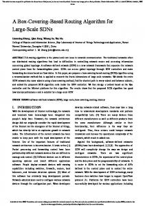
In Fig. 4(a), for both SF-DCLC and LCLD algorithms, the number of lost packets is plotted. It is clear that the proposed LCLD algorithm has less packet loss than the SF-DCLC algorithm. Fig. 4(b) shows the total number of received packets versus simulation time. According to the results shown in this figure, the number of received packets in LCLD is larger than SF-DCLC algorithm. Furthermore, in Fig. 4(c) and Fig. 4(d), the throughput and the end to end delay of both algorithms are plotted versus simulation time. It is clear that the proposed LCLD can outperform the SF-DCLC algorithm. 140

SF-DCLC

130

LCLD

120 110 100 90 80 0

20

40

(a) 60000

SF-DCLC

55000

LCLD

50000 45000 40000 35000 30000 25000 20000 0

20

40

sim ulation tim e

(b)

Fig. 3. Network topology in the nam environment

We have done four simulation trials. In the first trial, the number of flow and Δ delay , were set to 20 and 15, respectively. For performance comparison, it is necessary for both two algorithms to route the same requests and the same subset of requests in the same order.

60

sim ulation tim e

number of packet received

vector received from its neighbors. Since a node at most has |V| neighbors and a vector from one neighbor contains |V| entries,

60

LCLD

11000

SF-DCLC

LCLD

number of packet loss

throughput(no. of packet/TIL)

12000

10000 9000 8000 7000

240 230 220 210 200 190 180 170 160 150

SF-DCLC

5

6000 0

5 10 simulation time

10

15

20

delay level

15

(a)

(c)

SF-DCLC

number of received packets

LCLD

End2End delay(sec)

0.04 0.035 0.03 0.025 0.02 0.015

LCLD

0.01

SF-DCLC

0.005

50000 40000 30000 20000 10000 0 0

5

10

15

20

delay level

0 5

10 simulation time

15

20

(d) Fig.4: Simulation results: a) number of lost packets b) number of received packets c) throughput d)end to end delay

In the second trial, we evaluate the performance of both algorithms at different level of delay constraint. In this case, Δ delay is randomly selected. The number of flow was set to 20. We observed that, when delay bound is very stringent, both of compared algorithms are very close. These results can be explained as follows. When delay constraint is stringent, the number of feasible paths is very limited. Both algorithms are likely to choose the same path, so their performance is similar to each other. However, when the delay constraint becomes loose, the number of feasible paths increases. Therefore their performance starts to diverge. We also observe that LCLD has better capability to find the optimal path than SF-DCLC. In Fig. 5(a), for both SF-DCLC and LCLD algorithms, the number of lost packets is plotted versus different delay level. It is clear that the proposed LCLD algorithm has less packet loss than the SF-DCLC algorithm. Fig. 5(b) shows the number of received packets versus different delay level. According to the results shown in this figure, the number of received packets in LCLD is larger than SF-DCLC algorithm.

(b) throughput(no. of packets/TIL)

0

14000

SF-DCLC

12000

LCLD

10000 8000 6000 4000 2000 0 5

10

15

delay level

(c)

20

LCLD

250

SF-DCLC

0.017

number of packet loss

end to end delay(sec)

0.018 0.016 0.015 0.014 0.013 0.012 0.011

230 210 LCLD

190

SF-DCLC

170 150

0.01 5

10

15

3

20

8

13 number of flow

delay level

(a)

In the third trial, we evaluate the performance of both algorithms at different number of flow. In this case the delay level is constant. By increasing the number of flows, the number of received packets at destination is also increased. Due to the lack of enough bandwidth, the total number of received packets will not be increased from a certain number. This is also true for throughput and number of lost packets. In Fig. 6(a), for both SF-DCLC and LCLD algorithms, the number of lost packets is plotted versus different number of flow. It is clear that the proposed LCLD algorithm has less packet loss than the SF-DCLC algorithm. Fig. 6(b), for both SF-DCLC and LCLD algorithms, shows the number of received packets versus different number of flow. According to the results shown in this figure, the number of received packets in LCLD is larger than SF-DCLC algorithm. In Fig. 6(c) the throughput of both algorithms is plotted versus number of flow. Furthermore, in Fig. 6(d), the end to end delay of both algorithms is plotted versus number of flow. By increasing the number of flows, as the chosen path has a fixed link delay, the end to end delay will not be changed a lot.

70000 65000 60000 55000 50000 45000 40000 35000 30000

SF-DCLC LCLD

3

8

13

18

number of flow

(b) throughput(no. of packets/TIL)

In Fig. 5(c) and Fig. 5(d), the throughput and the end to end delay of both algorithms are shown. It can be seen that by increasing the delay level, limitation on the constraint of delay is decreased and some paths with extremely less cost and more delay may be chosen, so end to end delay is also increased.

number of received packets

(d) Fig. 5: Simulation results for different delay level: a) number of lost packets b) number of received packets c) throughput d) end to end delay

18

11000 10000 9000 8000 7000

SF-DCLC

6000

LCLD

5000 4000 3

8

13 number of flow

(c)

18

(a) 204000 number of received packets

end to end delay(sec)

0.025 0.023 0.021 0.019

SF-DCLC LCLD

0.017 0.015 3

8

13

18

184000

LCLD

164000

SF-DCLC

144000 124000 104000 84000 64000 44000

number of flow

1

3

5

7

number of source-destination

(d)

number of (source, destination) pairs will cause the increment of the chosen paths and traffic in the network. So, the total number of received packets in all destination’s nodes will be increased. In Fig. 7(a) , for both SF-DCLC and LCLD algorithms, the number of lost packets is plotted versus number of (source,destination) pairs. It is clear that the proposed LCLD algorithm has less packet loss than the SF-DCLC algorithm. Fig. 7(b) shows the total number of received packets. According to the results shown in this figure, for different number of (source,destination) pairs, the number of received packets in LCLD is larger than SF-DCLC algorithm. Fig.7(c) shows the throughput of both algorithms. Fig. 7(d) shows end to end delay. Based on results shown in these figures, It is clear that at different number of (source,destination) pairs, the proposed LCLD has better performance than SF-DCLC algorithm.

throughput(no. of packet/TIL)

In the last trial, we evaluate the performance of both algorithms at different number of (source,destination) pairs in the network. In this case, like to trial1, the number of flow and Δ delay , were set to 20 and 15, respectively. the Increasing the

(b) 28000 26000 24000 22000 20000 18000 16000 14000 12000 10000

SF-DCLC LCLD

1

3

5

7

number of source-destination

(c)

0.1 End to End Delay(sec)

Fig. 6: Simulation results for different number of flows: a) number of lost packets b) number of received packets c) throughput d)end to end delay

SF-DCLC LCLD

0.08 0.06 0.04

number of packet loss

0.02 1

200 190

LCLD

180 170

3

5

7

number of source-destination

SF-DCLC

160 150 140

(d)

130 120

Fig. 7: Simulation results with various (source,destination) pairs: a) number of lost packets b) number of received packets c) throughput d) end to end delay

1

3

5

7

num ber of source-destination

V.

CONCLUSION

In this paper, we studied the SF-DCLC problem, which is crucial for the emerging delay-cost sensitive applications. We proposed a distributed unicast routing algorithm, namely, LCLD, based on a special heuristic weight function. We also evaluated our algorithm by comparing it with SF-DCLC in terms of optimality. Our simulation results show that LCLD has much better performance than SF-DCLC. Thus, the most attractive feature of the LCLD algorithm is its high efficiency in the sense that it has very high probability of finding the optimal path with very low complexity. The worst-case computational complexity of this algorithm, for a network graph with v nodes, is equal with O(|v|2).

VI. [1] [2] [3]

[4] [5] [6] [7]

[8] [9] [10] [11] [12] [13]

[14] [15] [16]

[17]

REFERENCES

S. Chen and K. Nahsted, “An overview of quality of service routing for next-generation high-speed network: problems and solutions,” IEEE Networks, 1998, 12, (6), pp. 64-79. A. Shaikh, J. Rexford, and K. G. Shin, “Evaluating the impact of stale link state on quality-of-service routing,” IEEE/ACM Transactions on Networking, 2001, 9, (2), pp. 162-176. E.Aboelela, and C. Douligeris, “Fuzzy reasoning approach for QoS routing in B-ISDN,” Journal of Intelligent and Fuzzy Systems, Application in Engineering and Technology, Vol. 9, pp. 11-27,November 2000. Gang Cheng and Nirwan Ansari , “Achieving 100% Success Ratio In Finding The Delay Constrained Least Cost Path, ”IEEE Journal 2004. Luis Henrique M.K. Costa Serge Fdida,” Developing Scalable for Three-Metric QOS-Routing ,” Elsevier 2002. Z. Wang, and J. Crowcroft, “Quality of service routing for supporting multimedia applications,” IEEE Journal of Selected Areas in Communications, vol. 14, issue 7, pp. 1288-1234, September 1996. L. H. M. K. Costa, S. Fdida, and O. C. M. B. Duarte, “ Distance-Vector QOS based routing with three metrics,” in IFIP High Performance Networking – Networking 2000, Lecture Notes in Computer Science 1815, pp.847-856, May 2000. L. H. M. K. Costa, S. Fdida, and O. C. M. B. Duarte, “ A scalable algorithm for link-state Qos-based routing with three metrics,” in IEEE International Conference on Communications, june 2001. R. Widyono, “The design and evaluation of routing algorithms for real-time channels,” Technical Report ICSI TR-94-024, International Computer Science Institute, UC, Berkeley, June 1994. D. H. Lorenz and A. Orda, ”Efficient QoS partition and routing of unicast and multicast,” Proceedings of 8th International Workshop on Quality of Service, pp. 75-83, 2001. R. Hassin, ”Approximation schemes for the restricted shortest path problem,” Mathematics of Operations Research, 1992, 2, (2), pp. 36-42. D. Raz, and Y. Shavitt, “Optimal partition of QoS requirements with discrete cost functions,” IEEE Journal on Selected Areas in Communications, 2000, vol. 12, (18), pp. 2593-2602. A. Iwata, R. Izmailov, D.-S. Lee, B. Sengupta, G.Ramamurthy, H. Suzuki, “ATM routing algorithm with multiple QoS requirements for multimedia internetworking,” IEICE Transactions and Communications E70-B (8) (1998) 999–1006. H. De Neve, P. Van Mieghem, “A multiple quality of service routing algorithm for PNNI,” in: Proceedings of the IEEE ATM Workshop, May 1998, pp. 324–328. P. Van Mieghem, H. De Neve, F.A. Kuipers, “Hop-by-Hop quality of service routing, “Computer Networks 37 (2001) 407–423. E.I. Chong, S. Maddila, S. Morley, “On finding single source single-destination k shortest paths,” in: Proceedings of International Conference on Computing and Information (ICCI)_95, July 1995, pp. 40–47. X. Yuan, “Heuristic algorithm for multi-constrained quality-of-service routing, ”IEEE/ACM Transactions on Networking 10 (2) (2002) 244–256.

[18] G. Liu, K.G. Ramakrishnan, “A*Prune: an algorithm for finding K shortest paths subject to multiple constraints,” in: Proceedings of IEEE INFOCOM 2001. [19] L. Guo, I. Matta, “ Search space reduction in QoS routing,” Computer Networks 41 (1) (2003) 73–88. [20] E.I. Chong, S. Maddila, S. Morley, “On finding single source single-destination k shortest paths,” in: Proceedings of International Conference on Computing and Information (ICCI)_95, July 1995, pp. 40–47. [21] A. Juttner, B. Szviatovszki, I. Mecs, Z. Rajko, “Lagrange relaxation based method for the QoS routing problem,” in: Proceedings of the IEEE INFOCOM_2001, vol. 2 ,pp. 859-868. [22] T. Korkmaz, M. Krunz, S. Tragoudas, “An efficient algorithm for finding a path subject to two additive constraints”, Joint International Conference on Measurement and Modeling of Computer Systems, Proceedings of the 2000 ACM SIGMETRICS, Santa Clara, California, United States, 2000. [23] G. Feng, C. Douligeris, K. Makki, N. Pissinou, “Performance Evaluation of the Delay-Constrained Least-Cost Routing Algorithms Based on Linear and Nonlinear Lagrange Relaxation”, Proceedings of Fiftieth IEEE International Conference on Communication (ICC 2002), pp 2273-2278, April 2002. [24] D.S. Reeves, H.F. Salama, “A distributed algorithm for delay-constrained unicast routing,” IEEE/ACM Transactions on Networking 8 (2) (2000) 230–250. [25] Q. Sun, H. Langendorfer,” A new distributed routing algorithm for delay-sensitive application,” Computer Communications 21 (6) (1998) 572–578. [26] K. Ishida, E. Amana, N. Kannari, “A delay-constrained least cost path routing protocol and the synthesis method,” in: Proceedings of the Fifth IEEE International Conference on Real-Time Computer System and Applications, October 1998, pp. 58–65. [27] R. Sriram, G. Manimaran, C.S. Murthy,” Preferred link based delay-constrained least-cost routing in wide area networks,” Computer Communications 21 (1998) 1655–1669. [28] S. Chen, K. Nahrstedt, “Distributed quality-of-service routing in ad-hoc networks,” IEEE Journal on Selected Areas in Communications 17 (8) (1999) 1488–1505. [29] L. Xiao, J. Wang, K. Nahrstedt,” The enhanced ticket based routing algorithm,” in: Proceedings of the of ICC_02, New York, April 2002. [30] Wei Liu a,*, Wenjing Lou b, Yuguang Fang,” An efficient quality of service routing algorithm for delay-sensitive applications,” of Elsevier Computer Networks 47(2005) 87-104. [31] NS-2 Network Simulator , http://www.isi.edu/nsnam/ns/ Maryam Baradran was born in Mashad, Iran. She received her B.S. degree in Computer Engineering from Azad University of Mashad and her M.S. degree from Azad University of Mashad in 2007. Currently she is a faculty staff of Azad University of Mashad.

Mohammad Hossein Yaghmaee was born on July 1971 in Mashad, Iran. He received his B.S. degree in Communication Engineering from Sharif University of Technology, Tehran, Iran in 1993, and M.S. degree in communication engineering from Tehran Polytechnic (Amirkabir) University of Technology in 1995. He received his PhD degree in communication engineering from Tehran Polytechnic (Amirkabir) University of Technology in 2000. He has been a computer network engineer with several networking projects in Iran Telecommunication Research Center (ITRC) since 1992. November 1998 to july1999, he was with Network Technology Group (NTG), C&C Media research labs., NEC Corporation, Tokyo, Japan, as visiting research scholar. He is author of two books. Furthermore, he has published more than 55 technical papers. His research interests are in traffic and congestion control, high speed networks including ATM and MPLS, Quality of Services (QoS) and fuzzy logic control.