A Constraint Seeker: Finding and Ranking Global Constraints from Examples Nicolas Beldiceanu1 and Helmut Simonis2? 1
Mines de Nantes, LINA UMR 6241, FR-44307 Nantes, France
[email protected] 2 Cork Constraint Computation Centre Department of Computer Science, University College Cork, Ireland
[email protected]
Abstract. In this paper we describe a Constraint Seeker application which provides a web interface to search for global constraints in the global constraint catalog, given positive and negative ground examples. Based on the given instances the tool returns a ranked list of matching constraints, the rank indicating whether the constraint is likely to be the intended constraint of the user. We give some examples of use cases and generated output, describe the different elements of the search and ranking process, discuss the role of constraint programming in the different tools used, and provide evaluation results over the complete global constraint catalog.
1
Motivation
The global constraint catalog [4] provides a valuable repository of global constraint information for both researchers in the constraint field and application developers searching for the right modelling abstraction. The catalog currently describes over 350 constraints on more than 2800 pages. This wealth of information is also its main weakness. For a novice (and even for an experienced) user it can be quite challenging to find a particular constraint, unless the name in the catalog is known. As a consistent naming scheme (like the naming scheme for chemical compounds http://en. wikipedia.org/wiki/IUPAC_nomenclature, for example) does not exist in the constraint field, and different constraint systems often use incompatible names and argument orders for their constraints, there is no easy way to deduce the name of a constraint and the way its arguments are organized from its properties. The catalog already provides search by name, or by keywords, and provides extensive cross-references between constraints, as well as a classification by the required argument type. All of these access methods can be helpful, but are of limited use if one does not know too much about the constraint one is looking for. The Constraint Seeker (http://seeker.mines-nantes.fr) provides another way of finding constraint candidates, sorted by potential relevance, in the catalog. The user provides positive and/or negative ground instances for a constraint, and the tool provides a ranked list of possible candidates which match the given examples. ?
Part of this work was created while the second author visited Nantes in 2010.
2
Related Work
Our Constraint Seeker is related to a number of other systems, and, more fundamentally, to a strand of research in constraints. 2.1
Integer Sequences
A key motivation for developing the Constraint Seeker was the example of an interactive website http://oeis.org/Seis.html for Integer Sequences [22]. In this tool, the user can enter a sequence of integer values, and the search tool will return a list of those integer sequences in its library which seem to match that sequence, either as a prefix, or as a subset of the values. Candidates are ranked by similarity to the example given, for example a prefix is considered more similar than a subset matching. 2.2
Constraint Taxonomy
Taxonomies (structure/sub-structure relations) are often used to give access to large collections of information, and form the basis of many on-line information retrieval systems. Unfortunately, there has been rather little work on providing a taxonomy of different constraints. A taxonomy considering only difference and equality is proposed in [15], while a taxonomy of the global constraints in the CHIP system was given in [21]. 2.3
Library Seeker
Library search tools for programming languages typically allow search by name and by a taxonomy of intended function. A search tool for CamlLight [26] at http://www. dicosmo.org/TESTS/ENGLISH/CamlSearchCGI.english.html also provides lookup by type. One can enter a type specification for a library function, and the system should return all library functions with isomorphic types.3 Using the signature of the constraint is an important element of our Constraint Seeker, as it allows to restrict the search to a relatively small subset of the complete catalog, while at the same time not requiring to guess the complete signature of the constraint. 2.4
Electronic Symbol Catalog
The interactive Electrical What catalog http://electricalwhat.com/ gives another example of a search tool, where just searching by name is not sufficient. The catalog lists images of electronic symbols, and the user can search by category (transistor, diode, etc), but also by structural properties of the symbol (how many connections, major symbol a circle, a rectangle or a triangle, etc). This is required by a use case where a novice sees a new symbol, but does not know what it stands for. This is quite similar to our use case of encountering a constraint, and describing its properties, instead of searching for it by name. 3
The system seems to be no longer operational.
2.5
Constraint Acquisition
Constraint Acquisition [17] is the process of finding a constraint network from a training set of positive and negative examples. The learning process operates on a library of allowed constraints, and a resulting solution is a conjunction of constraints from that library, each constraint ranging over a subset of the variables. This area of research has attracted a fair bit of work over the last ten years [8, 24, 6, 16, 5, 14, 7, 13, 18, 20, 19]. A key idea for solving this problem is the use of version space learning from AI, which considers the set of all possible constraint networks which accept the training set. In an interactive setting, the training set is not fixed, but will be derived incrementally. If the target model has not been identified, the system may suggest new training instances, which the user has to classify as either positive or negative. Ideally, these new examples are chosen to maximally reduce the version space that needs to be considered. One of the challenges of constraint acquisition for a library of global constraints is that many global constraints have additional parameters which might not occur in the examples given, which only list the main decision variables describing the problem. The values of these parameters must be learned from the examples as well, this is considered in [9, 10]. Another issue is that in constraint acquisition we don’t know over which subset of the decision variables a constraint will be expressed. When we consider only binary constraints, this does not matter, we can explore all binary combinations of variables in quadratic time. For a global constraint with k variables which ranges over a subset of n decision variables, we are faced with a combinatorial explosion, especially if the order of the variables in the constraint matters. Our problem of the Constraint Seeker is closely related to the constraint acquisition problem, but subtly different. We are not looking for a model of a complete constraint problem, we are searching for a single constraint in the global constraint catalog. It means that we know the variables over which the constraint ranges, as well as their order in a collection, and we assume that most (but not necessarily all) additional parameters are given as well. This makes it possible to search over the complete catalog of 350+ constraints without a combinatorial explosion.
3
User Experience
We now show the behaviour of the Constraint Seeker on a simple example. The user interacts with the system through a simple web form, where he must give at least one positive example for the constraint. Suppose the user enters the query p( 2 , [4,2,4,5] , 4 ) where p stands for positive example. The colors for the arguments are applied by the Seeker to help visualize changes in the argument order in the output. 3.1
Seeker Matches
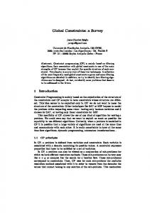
Figure 1 shows the output of the Constraint Seeker for the sample query, formatted for pdf output.
Fig. 1. Example Output of Constraint Seeker for Query p( 2 , [4,2,4,5] , 4 ) Constraint exactly
Rank Density Links UnTyp ArgOrder Crisp Func Tr 0 3125 9 0 0 n/a graph Pattern: exactly( 2 , [[var-4],[var-2],[var-4],[var-5]] , 4 ) exactly implies atmost Relations: exactly implies atleast atleast 5 5625 11 0 0 0 n/a Pattern: atleast( 2 , [[var-4],[var-2],[var-4],[var-5]] , 4 ) Relations: atleast implied by exactly atmost 5 9188 12 0 0 0 n/a Pattern: atmost( 2 , [[var-4],[var-2],[var-4],[var-5]] , 4 ) Relations: atmost implied by exactly minimum greater than 30 2146 10 0 3 n/a n/a Pattern: minimum greater than( 4 , 2 , [[var-4],[var-2],[var-4],[var-5]] ) int value precede 30 7060 11 0 3 n/a n/a Pattern: int value precede( 4 , 2 , [[var-4],[var-2],[var-4],[var-5]] ) atmost 30 9188 12 1 2 3 n/a Pattern: atmost( 4 , [[var-4],[var-2],[var-4],[var-5]] , 2 ) Relations: atmost implied by exactly
In the output the candidate explanations are listed by relevance, i.e. for the given example the first entry, the exactly constraint, is the best explanation. It has rank 0, a numerical value computed from structural information about the candidate. The density value (3125) shows how many solutions were counted for a small instance of the constraint, constraints with few solutions are more likely candidate explanations than constraints with many solutions. The exactly constraint has 9 links, i.e. its description refers to nine other constraints in the catalog. Constraints with many links are typically more common and useful, e.g. alldifferent has 72 links. The exactly constraint is also marked as having a functional dependency. One of the arguments (the first) is determined by the values for the other arguments, as we are counting in the first argument how often a particular value (the third argument) occurs in a list of values (the second argument). Constraints with functional dependencies are considered good candidate explanations, therefore the rank value for the exactly constraint is very low. The functional dependency is derived from the graph description [1] of the constraint in the catalog, i.e. it was not specified manually. For other constraints this property can be deduced from the specification of the constraint as an automaton [2], but for some of the constraints (mostly numerical constraints) we had to define this property manually as meta-data in the catalog. The second line of the exactly constraint shows the actual call pattern that must be used, in this case the user input is used without any transformation. The Constraint Seeker does allow for permutations of the arguments, and even within list arguments,
since it is not reasonable to require that a user knows the particular argument order used in the catalog. The third line shows relations between the exactly constraint and other candidates found. The exactly constraint implies both the atleast and the atmost constraint, it is therefore a better (more specific) candidate explanation and ranked above the other candidates. The second candidate shown is the atleast constraint, with a rank of 5 and a density of 5625. Its rank must be greater than that of the exactly constraint, as atleast is implied by exactly, but it is also influenced by what we call crispness of its first argument. In the atleast constraint, the first argument is not a functional dependency of the other arguments, but it is monotonic. If the constraint is satisfied for some value k in the first argument, it is also satisfied for all values smaller than k. The crispness of the constraint (column Crisp) is the difference between the maximal value for the argument that satisfies the constraint and the value that occurs in the user given pattern. Candidates with small crispness values are considered good explanations. The third candidate is atmost, which also has a rank of 5, but a density value of 9188, and which therefore is ranked lower than atleast.4 The next two candidates minimum greater than and int value precede require a permutation of their arguments to match the example instance given by the user, and have neither a functional dependency nor a monotonic argument. This leads to a relatively bad ranking value. The number of arguments that need to be permuted is given in the column ArgOrder. The last candidate is another variation of the atmost constraint. Instead of stating that atmost 2 values in the collection have value 4, this candidate explanation says that atmost 4 variables in the collection have value 2. This requires two argument swaps (ArgOrder=2), but also shows a crispness value of 3. In the instance given only one variable has value 2, so the first argument with its value 4 is three steps off the crisp value. This candidate also shows another issue, one of the typical restrictions for atmost is violated. The typical restrictions state conditions which hold in normal use of a constraint. For the atmost(N,Variables,Value) constraint, these restrictions are given in the catalog: 1. 2. 3. 4.
N >0 N < |VARIABLES | |VARIABLES | > 1 atleast(1, VARIABLES , VALUE )
Restriction 2 is not satisfied, as the collection contains only four variables, and the first argument N is also set to 4. Candidates which violate typical restrictions are considered weak explanations, and are therefore down-ranked. Wider Matches The candidates above were found by looking for explanations with the same compressed type as the example given, i.e. where the arguments were permutations of the user example. The Seeker can find more general examples, where the 4
This difference in solutions counted will become clear when, in Section 5.2, we describe the method for computing the density.
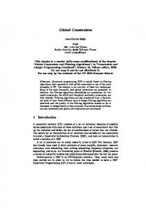
user input must be transformed in a more complex way to find the explanation. Typical cases are optional arguments which may or may not be present, reorganization of the arguments (a matrix for example may be given as a matrix, or as a collection describing the rows, or as a collection describing the columns). The two wider matches in the output in Figure 2 show explanations based on such transformations: In the first case, we find a match for element, based on a shift of an index argument. The global constraint catalog assumes that indices are counted from 1. Some constraint systems (like Choco or Gecode) instead follow their host language and count indices from 0. To match examples intended for such systems, we try to add one to index arguments. If we change the first argument from 2 to 3, then the instance matches an element constraint. This is the same as considering the constraint with the index in the first argument being counted from 0. The second candidate, count, is obtained by adding an additional argument with the equality operator. The user may not have considered parametrizing his example with such an operator, we therefore try to add this argument and try out all possible operator values, but only keep the strongest (most restrictive) of the possible choices.
Fig. 2. Extended Search Results Constraint Rank Density Links UnTyp ArgOrder Crisp Func Tr element 0 2500 35 0 0 n/a manual T11 Pattern: element( 3 , [[value-4],[value-2],[value-4],[value-5]] , 4 ) count 30 3125 16 0 3 n/a n/a T1 Pattern: count( 4 , [[var-4],[var-2],[var-4],[var-5]] , = , 2 )
Note that the ranking for element would place it at the top of the list if both result lists are combined. This is due to the functional dependency in the element constraint (the third argument is determined by the index and the list of values), and the small number of solutions it admits. The column Func indicates the functional dependency as manual, i.e. this is specified explicitly in the description of the constraint. Also note how the modified value in the first argument of element is highlighted, as well as the added argument in the count constraint. This matching of the arguments against the original example instance is done by a small constraint program, which also deals with new or modified arguments.
4
Generating Candidates
Given a set of positive and negative examples, we first have to find candidate explanations, constraints that match these examples. This requires the following steps: – We first construct a type signature from the examples, using the following ground types (page 6-8 of [4]) in the given lexicographical order: atom ≺ int ≺ real ≺ list ≺ collection
– We sort the arguments and collections in lexicographical order to generate a normalized type. – If we partition the constraints in the catalog by their normalized type signature, we find 97 distinct types, with the largest equivalence class containing 40 constraints (see page 109 of [4]). – For each constraint in the selected equivalence class we have to evaluate it against all positive and negative examples. In order to do this, we have to permute the examples given to create the call pattern matching the argument order of each constraint. There can be multiple ways to do this, for example if a constraint has multiple arguments of the same type, and we have to explore each of those possibilities. Fortunately, the number of permutations to be considered is often quite limited, there are only 15 constraints in the catalog for which we have to consider more than 72 permutations. – Different permutations can lead to the same call pattern, if for example multiple arguments have the same value. In other cases, the catalog explicitly provides the information that some arguments in the constraint are interchangeable (page 19 in [4]), i.e. there are symmetries which we don’t have to present multiple times. We can filter such duplicates before (or sometimes only after) the ranking of the candidate list. – In many cases we want to consider more than just a strict matching of the argument types. The user may present the arguments in a different form, e.g. use a matrix rather than a collection of collections. He might also have ignored or added some arguments, or optional parameters. We deal with these possibilities by using a rule-based transformation system which, based on pre- and post conditions, can modify the argument structure of the examples given. At the moment we use 13 such rules in the system (http://seeker.mines-nantes.fr/ transformations.htm). The process above results in a set of call pattern in the correct format for every constraint with the correct compressed type. In order to evaluate these pattern, we need some code that can check if these ground instances satisfy the constraint. In principle, we only need a constraint checker, which operates on a ground instance, and returns true or false. But the catalog descriptions may contain stronger implementations: built-in The Seeker code is executed in SICStus Prolog [12], which contains a finite domain solver that implements a number of global constraints. We can call these built-ins to execute the constraint, after some syntactic transformation. reformulation The constraint can be evaluated by executing a Prolog program which calls other global constraints and possibly some general Prolog code to transform arguments. Obviously, the call tree must not be cyclic, i.e. any constraints called may not use a reformulation which calls the initial constraint. automaton The constraint can be evaluated by an automaton with counters [3]. These can be executed directly in SICStus Prolog. logic An evaluator is provided as a logic based formula in the rule language extending the geost constraint described in [11]. An evaluator for the rule language is available in SICStus Prolog.
checker A small number of complex constraints (e.g. cycle) are described only with a constraint checker, which can evaluate ground instances only. While this is sufficient for the candidate generation, this will not be enough for other elements of the overall Seeker application. none No evaluator for the constraint is given in the catalog. For some constraints, multiple evaluators are given. Table 1 shows the current state of evaluators for the global constraint catalog. 274 of 354 (77.4%) can be evaluated. Most of the missing constraints use finite set variables or are graph constraints, which are not provided in the SICStus Prolog constraint engine.
Table 1. Evaluators for Global Constraints Evaluator Nr Constraints reformulation 137 automaton 49 reformulation + automaton 40 builtin 26 logic 9 builtin + automaton 8 checker 3 reformulation + reformulation 1 builtin + reformulation 1 none 80 Total 354
5
Ranking
Not all candidate explanations are equally useful to the user. We use three criteria to order the candidates, the rank being the most important, and the number of links the least important tie breaker: rank The rank of the constraint indicates how specific it is. The relative rank value is determined on-line by a constraint program which compares all candidates with each other. density We compute a solution density for each constraint by enumerating all solutions for small problem instances. Constraints with few solutions are considered better explanations. The solution density is pre-computed by another constraint program. links The number of cross references between constraints in the catalog gives an indication of their popularity.
5.1
Rank Computation Solver
The rank computation solver is run on-line for each query to produce a relative position for each candidate. The rank for each candidate is represented by a domain variable, small values are better than large ones. We use unary and binary constraints in this model. Unary constraints affect the lower bound of the domain variable based on a combination of: functional dependency If one or multiple arguments of a constraint depend on other arguments, it is quite unlikely that a user did pick the correct value by chance. Candidates with functional dependencies are good explanations. crispness Slightly weaker than functional dependencies, the crispness is derived from monotonic arguments. If the constraint holds for some value k of such an argument, it must also hold for all values larger (smaller) than k. We call the minimal (maximal) value for which the constraint holds, its crisp value. The smaller the difference between the crisp value and the value given in the example, the better is the candidate explanation. typical restriction violations For each constraint, the catalog describes restrictions which apply to a typical use of the constraint. If a candidate violates these typical restrictions, it should not be considered a good explanation, and it should be down ranked. argument reordering If the user has given the arguments of the constraint in the correct order, so that no re-ordering is required, we consider the constraint a better candidate than one where all arguments must be permuted. This is a rather weak criteria, as it is based on convention rather than structure. The exact formula on how these criteria are combined to affect the lower bound is based on a heuristic evaluation of different parameter choices. Binary constraints are imposed between candidate constraints for which semantic links (page 84 of [4]) are given in the catalog. As we had seen in our example in Section 3, the exactly constraint implies both atleast and atmost constraints. It is therefore a better candidate, and we impose inequality constraints between all candidates for which such semantic links exist. At the moment we only use the implies and implied by links, the links generalization and soft variant do not seem to work as well between constraints of the same call pattern. We search for a solution which minimizes the sum of all rank variables, this solution can be found by assigning the variables by increasing lower bound and fixing the smallest value in each domain. No backtracking is required. As a constraint problem this is not very difficult, the main advantage that CP gives is the flexibility with which different scenarios can be explored without much effort. 5.2
Density Solver
The solution density of each constraint is estimated off-line by two constraint models, and stored result values are then used in the on-line queries. Unfortunately, closed form formulas for solution counting are known for very few constraints [27], and thus can not be used in the general case. Instead, we create small problem instances only: For a
given size parameter n, we enumerate all argument pattern where all collections have n or fewer entries. For many constraints, the length of the collections is constrained by restrictions provided in the catalog, so that these choices can not be made arbitrarily. A small constraint program considers all these restrictions, by enumeration we find all combinations which are allowed. Having fixed the size of the collections in the first model the second model creates domains ranging from 0 to n, calls the constraint and enumerates all solutions with a timeout. The value 0 is included in the domain, as it often plays a special role in the constraint definition. In our experiments we restrict n to 4 or 5. Note that by imposing the “typical” restrictions in our models, we can also count how many typical solutions exist for a given constraint.
6
Instance Generation
The two models of the density solver can be used for another purpose. We can also generate positive instances for the constraints. In this variant, we change the domain limits from −2n to 2n, allow larger values for n, and use a more complex search routine, which tries to sample the complete solution space. The search routine first tries to assign some regular instances pattern, like setting each collection to all zero values, or enforcing monotonicity in some argument. In a second step, we try to set randomly selected arguments to random values. In a last step, we try to find instances for missing values. If in the previous phase some value has not been chosen for some argument, we try to force that value, in order to increase variety in the solution set. All phases are linked to time-outs, set to finish the complete catalog overnight. We can again impose the typical restrictions in order to find typical examples. We will use these randomly generated instances in our evaluation to compare against the manually chosen examples in the catalog.
7
Constraint Solving inside the Seeker
We have seen that the complete Constraint Seeker tool uses constraint models for multiple roles: 1. 2. 3. 4. 5. 6.
Check positive and negative examples for satisfaction (on-line) Rank candidate lists by estimated relevance (on-line) Determine the argument order used for output coloring (on-line) Compute all call patterns up to given size (off-line) Count all (typical) solutions for small problem sizes (off-line) Sample solution space to generate positive (typical) instances (off-line)
Each of these models is quite small, sometimes only involving the constraint under test. In other cases, various other constraints, from the typical restrictions for example, will be added. The search complexity ranges from trivial (ranking solver without backtracking), to quite complex (instance generator). Note that all of these models are generated automatically from the meta-data given in the catalog description. This means in particular that we generate typical and non-typical test cases for many global constraints solely from the abstract description in the catalog.
8
Evaluation
We have tested the Constraint Seeker against different example datasets: Catalog Examples The first set uses the examples which are given for each constraint in the catalog. For the vast majority of constraints, only a single positive instance is given, which was manually designed as part of the constraint description. We either use all tests for which an evaluator exists (Column all), only those for which we were able to also generate tests (Column restricted), or (Column first) only the first example given in the restricted set. Generated The second set uses the generated examples described in section 6. The order of the instances for each constraint is randomized. Instances can normally only be generated if an efficient evaluator for the constraint is available. Representatives We try to reduce the number of examples for each constraint, while maintaining some variety. Many generated examples produce the same candidate set. In this set we only use one representative from each such group. Single We pick a single, best test from the generated examples, i.e. one which minimizes the number of candidates and which has the highest ranking for the intended constraint. Combined We also pick a single best test, but this time from both the hand-crafted and the generated examples. In a first test we only check how many candidates are generated when running over all provided instances, and ignore the ranking. The numbers indicated in row k of table 2 state for how many constraints the Seeker found k candidates. The examples from the Table 2. Number of Candidates Generated Nr Catalog Examples Generated Representative Single Combined all restricted first Examples Examples 1 66 63 63 155 140 96 107 2 35 28 28 48 60 59 45 3 27 25 20 23 24 33 29 4 32 31 28 11 13 22 27 5 26 24 22 8 9 11 11 6 30 30 32 6 5 12 11 7 15 15 16 1 2 7 10 8 11 9 9 2 2 7 7 9 12 12 12 1 4 3 10 7 7 7 2 3 11 7 7 7 12 2 2 2 13 2 2 2 14 7 2 2
catalog produce up to 14 candidates, while for the generated examples and for the representative set up to nine candidates are produced. We can also see that the generated
examples are much more selective. For 155 constraints, there is only one candidate left. This drops to 140 constraints, if we only consider representatives, but that is still more than twice the number of examples with a single candidate when using the hand-crafted examples from the catalog. If we only consider a single test example, the generated examples do not fare quite as well, but still better than the hand-crafted examples. Combining both sets brings further improvements, showing that the hand-crafted examples are not always worse than the generated ones. Overall, we can see that the number of candidates is not excessive in any of the test scenarios, but that it is clearly not enough to just produce the candidate list. We now consider how good the ranking is at identifying the intended constraint. Table 3 shows in row only for how many constraints we get a single candidate which identifies the constraint. In that case the ranking is irrelevant. The next rows (first, second, third) indicate for how many constraint the ranking puts the correct constraint in first, second or third place. The next line (other) indicates that the intended constraint was not in the top three entries. The last row gives the total number of constraints identified for each dataset. The candidate selection together with the ranking produces rather Table 3. Quality of Ranking Nr Catalog Examples Generated Representative Single Combined all restricted first Examples Examples only 66 63 63 155 140 96 107 first 149 142 135 89 99 124 121 second 33 27 31 10 14 25 17 third 12 11 13 0 0 6 6 other 13 12 13 1 2 5 4 total 273 255 255 255 255 255 255
strong results for the generated examples. For 244 of 255 constraints do we find the intended constraint in first position, only in 11 of 255 (4.3%) case do we not find the intended constraint at the top of the candidate list, and in only one case it is not in the top three. This increases to 16 of 255 (6.2 %) cases for the representative set, and to 35 of 255 (13.7%) if we pick only one example. The hand-crafted examples are somewhat weaker, in 58 of 273 cases (21.2 %) do we not find the intended constraint in first position. Picking a single, best example from both generated and hand-crafted examples leaves us with 27 of 255 cases not identified in first position (10.6 %), but only 4 cases (1.6 %) not in the top three. We can also provide some analysis at the system level. The Constraint Seeker is written in SICStus Prolog, integrated with an Apache web server. Nearly all of the HTML output is generated, the rest is fairly simple forms and css data. The Prolog code is just over 6,400 lines, developed over a period of 3 months by one of the authors. The six constraint models in the Seeker make up 2,000 lines, roughly one third of the code. This line count does not include the 50,000 lines of Prolog describing the constraints themselves. This description is not specific to the Seeker, instead it provides the meta
data that systematically document the various aspects of the global constraints, while its first use was to generate the textual form of the catalog itself.
9
Summary and Future Work
Besides introducing the Constraint Seeker, the key contribution of the paper is to illustrate the power of meta data and meta programming in the context of future constraints platforms. Constraint platforms today typically provide some or all of the following features: 1. 2. 3. 4. 5.
The core engine dealing with domains, variables and propagation. A set of built-in constraints with their filtering algorithms. Some generic way to define new constraints (e.g. table, MDD, automata). A low level API to define new constraints and their filtering algorithms. A modelling language which may also allow to express reformulation.
However, it is well known that a lot of specific knowledge is required for achieving automatically various tasks such as validating constraints in a systematic way, breaking symmetries, or producing implied constraints. To deal with this aspect we suggest a complementary approach where we use meta data for explicitly describing different aspects of global constraints such as argument types, restrictions on the arguments, typical use of a constraint, symmetries w.r.t. the arguments of a constraint, links between constraints (e.g. implication, generalisation). The electronic version of the global constraint catalog provides such information in a systematic way for the different global constraints. The Constraint Seeker presented in this paper illustrates the fact that the same meta data can be used for different purposes (unlike ad-hoc code in a procedural language which is designed for a specific (and unique) usage and a single system). In fact to build our Constraint Seeker we have systematically used the meta data describing the constraints for solving a number of dedicated problems such as: – Estimating the solution density of a constraint, which was needed for the ranking. – Extracting structural information about a constraint from meta data (e.g. functional dependency between the arguments of a constraint) used for the ranking. – Generating discriminating examples for all constraints, as well as typical examples with some degree of diversity for systematically evaluating our Constraint Seeker. – Using the symmetry information for automatically filtering out symmetrical answers of the Constraint Seeker. Beside these problems, the meta data is also used for generating the catalog. It is worth noting that it could also be used for simulating the effect of various consistencies, getting interesting examples of missing propagation, and providing certificates for testing constraints for all constraints of the catalog. The key point to keep in mind is that with this approach it is possible to design a variety of tools that don’t need to be updated when new constraints are added (i.e., we only need to provide meta data for the new constraint as well as an evaluator). This contrasts with today’s approach where constraint libraries need to modify a number of things as soon as a new constraint is added
(e.g. update the manual, write specific code for testing the parameters of the constraint, generate meaningful examples, update the test cases, . . . ). The current version of the Constraint Seeker has been deployed on the web (http: //seeker.mines-nantes.fr), future work will study queries given by the users to identify further improvements of the user experience.
References 1. N. Beldiceanu. Global constraints as graph properties on a structured network of elementary constraints of the same type. In R. Dechter, editor, Principles and Practice of Constraint Programming (CP’2000), volume 1894 of LNCS, pages 52–66. Springer-Verlag, 2000. Preprint available as SICS Tech Report T2000-01. 2. N. Beldiceanu, M. Carlsson, R. Debruyne, and T. Petit. Reformulation of global constraints based on constraint checkers. Constraints, 10(3), 2005. 3. N. Beldiceanu, M. Carlsson, and T. Petit. Deriving filtering algorithms from constraint checkers. In Wallace [25], pages 107–122. 4. N. Beldiceanu, M. Carlsson, and J. Rampon. Global constraint catalog (second edition). Technical Report T2010:07, SICS, 2010. 5. C. Bessi`ere, R. Coletta, E. C. Freuder, and B. O’Sullivan. Leveraging the learning power of examples in automated constraint acquisition. In Wallace [25], pages 123–137. 6. C. Bessi`ere, R. Coletta, F. Koriche, and B. O’Sullivan. A SAT-based version space algorithm for acquiring constraint satisfaction problems. In J. Gama, R. Camacho, P. Brazdil, A. Jorge, and L. Torgo, editors, ECML, volume 3720 of Lecture Notes in Computer Science, pages 23–34. Springer, 2005. 7. C. Bessi`ere, R. Coletta, F. Koriche, and B. O’Sullivan. Acquiring constraint networks using a SAT-based version space algorithm. In AAAI. AAAI Press, 2006. 8. C. Bessi`ere, R. Coletta, B. O’Sullivan, and M. Paulin. Query-driven constraint acquisition. In Veloso [23], pages 50–55. 9. C. Bessi`ere, R. Coletta, and T. Petit. Acquiring parameters of implied global constraints. In P. van Beek, editor, CP, volume 3709 of Lecture Notes in Computer Science, pages 747–751. Springer, 2005. 10. C. Bessi`ere, R. Coletta, and T. Petit. Learning implied global constraints. In Veloso [23], pages 44–49. 11. M. Carlsson, N. Beldiceanu, and J. Martin. A geometric constraint over k-dimensional objects and shapes subject to business rules. In P. J. Stuckey, editor, CP, volume 5202 of Lecture Notes in Computer Science, pages 220–234. Springer, 2008. 12. M. Carlsson et al. SICStus Prolog User’s Manual. Swedish Institute of Computer Science, release 4 edition, 2007. ISBN 91-630-3648-7. 13. J. Charnley, S. Colton, and I. Miguel. Automatic generation of implied constraints. In G. Brewka, S. Coradeschi, A. Perini, and P. Traverso, editors, ECAI, volume 141 of Frontiers in Artificial Intelligence and Applications, pages 73–77. IOS Press, 2006. 14. R. Coletta, C. Bessi`ere, B. O’Sullivan, E. C. Freuder, S. O’Connell, and J. Quinqueton. Semiautomatic modeling by constraint acquisition. In F. Rossi, editor, CP, volume 2833 of Lecture Notes in Computer Science, pages 812–816. Springer, 2003. 15. E. Hebrard, D. Marx, B. O’Sullivan, and I. Razgon. Constraints of difference and equality: A complete taxonomic characterisation. In I. P. Gent, editor, CP, volume 5732 of Lecture Notes in Computer Science, pages 424–438. Springer, 2009. 16. S. O’Connell, B. O’Sullivan, and E. C. Freuder. Timid acquisition of constraint satisfaction problems. In H. Haddad, L. M. Liebrock, A. Omicini, and R. L. Wainwright, editors, SAC, pages 404–408. ACM, 2005.
17. B. O’Sullivan. Automated modelling and solving in constraint programming. In M. Fox and D. Poole, editors, AAAI. AAAI Press, 2010. 18. J. Quinqueton, G. Raymond, and C. Bessiere. An agent for constraint acquisition and emergence. In V. Negru, T. Jebelean, D. Petcu, and D. Zaharie, editors, SYNASC, pages 229–234. IEEE Computer Society, 2007. 19. F. Rossi and A. Sperduti. Acquiring both constraint and solution preferences in interactive constraint systems. Constraints, 9(4):311–332, 2004. 20. K. M. Shchekotykhin and G. Friedrich. Argumentation based constraint acquisition. In W. Wang, H. Kargupta, S. Ranka, P. S. Yu, and X. Wu, editors, ICDM, pages 476–482. IEEE Computer Society, 2009. 21. H. Simonis. Building industrial applications with constraint programming. In H. Comon, C. March´e, and R. Treinen, editors, CCL, volume 2002 of Lecture Notes in Computer Science, pages 271–309. Springer, 1999. 22. N. J. A. Sloane and S. Plouffe. The Encyclopedia of Integer Sequences. Academic Press, San Diego, 1995. 23. M. M. Veloso, editor. IJCAI 2007, Proceedings of the 20th International Joint Conference on Artificial Intelligence, Hyderabad, India, January 6-12, 2007, 2007. 24. X. Vu and B. O’Sullivan. Generalized constraint acquisition. In I. Miguel and W. Ruml, editors, SARA, volume 4612 of Lecture Notes in Computer Science, pages 411–412. Springer, 2007. 25. M. Wallace, editor. Principles and Practice of Constraint Programming - CP 2004, 10th International Conference, CP 2004, Toronto, Canada, September 27 - October 1, 2004, Proceedings, volume 3258 of Lecture Notes in Computer Science. Springer, 2004. 26. P. Weis and X. Leroy. Le langage Caml. InterEditions, 1993. in French. 27. A. Zanarini and G. Pesant. Solution counting algorithms for constraint-centered search heuristics. Constraints, 14(3):392–413, 2009.