A Continuum Mechanical Approach to Geodesics in ... - CiteSeerX

A Continuum Mechanical Approach to Geodesics in Shape Space Benedikt Wirth† Leah Bar‡ Martin Rumpf† Guillermo Sapiro‡ † Institute for Numerical Simulation, University of Bonn, Germany ‡ Department of Electrical and Computer Engineering, University of Minnesota, Minneapolis, U.S.A. Abstract In this paper concepts from continuum mechanics are used to define geodesic paths in the space of shapes, where shapes are implicitly described as boundary contours of objects. The proposed shape metric is derived from a continuum mechanical notion of viscous dissipation. A geodesic path is defined as the family of shapes such that the total amount of viscous dissipation caused by an optimal material transport along the path is minimized. The approach can easily be generalized to shapes given as segment contours of multi-labeled images and to geodesic paths between partially occluded objects. The proposed computational framework for finding such a minimizer is based on the time discretization of a geodesic path as a sequence of pairwise matching problems, which is strictly invariant with respect to rigid body motions and ensures a 1-1 correspondence along the induced flow in shape space. When decreasing the time step size, the proposed model leads to the minimization of the actual geodesic length, where the Hessian of the pairwise matching energy reflects the chosen Riemannian metric on the underlying shape space. If the constraint of pairwise shape correspondence is replaced by the volume of the shape mismatch as a penalty functional, one obtains for decreasing time step size an optical flow term controlling the transport of the shape by the underlying motion field. The method is implemented via a level set representation of shapes, and a finite element approximation is employed as spatial discretization both for the pairwise matching deformations and for the level set representations. The numerical relaxation of the energy is performed via an efficient multi-scale procedure in space and time. Various examples for 2D and 3D shapes underline the effectiveness and robustness of the proposed approach.

1

Introduction

In this paper we investigate the close link between abstract geometry on the infinite-dimensional space of shapes and the continuum mechanical view of shapes as boundary contours of physical objects in order to define geodesic paths and distances between shapes in 2D and 3D. The computation of shape distances and geodesics is fundamental for problems ranging from computational anatomy to object recognition, warping, and matching. The aim is to reliably and effectively evaluate distances between non-parametrized geometric shapes of possibly different topology. In particular, we allow shapes to consist of boundary contours 1

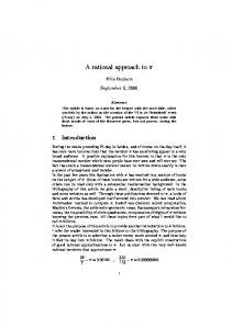
Figure 1: Time-discrete geodesic between the letters A and B. The geodesic distance is measured on the basis of viscous dissipation inside the objects (color-coded in the top row from blue, low dissipation, to red, high dissipation), which is approximated as a deformation energy of pairwise 1-1 deformations between consecutive shapes along the discrete geodesic path. Shapes are represented via level set functions, whose level lines are texture-coded in the bottom row. of multiple components of volumetric objects. The underlying Riemannian metric on shape space is identified with physical dissipation (cf. Fig. 1)—the rate at which mechanical energy is converted into heat in a viscous fluid due to friction—accumulated along an optimal transport of the volumetric objects (cf. [47]). We simultaneously address the following major challenges: A physically sound modeling of the geodesic flow of shapes given as boundary contours of possibly multi-component objects on a void background, the need for a coarse time discretization of the continuous geodesic path, and a numerically effective relaxation of the resulting time- and space-discrete variational problem. Addressing these challenges leads to a novel formulation for discrete geodesic paths in shape space that is based on solid mathematical, computational, and physical arguments and motivations. Different from the pioneering diffeomorphism approach by Miller et al. [35] the motion field v governing the flow in shape space vanishes on the object background, and the accumulated physical dissipation is a quadratic functional depending only on the first order local variation of a flow field. In fact, as we will explain in a separate section on the physical background, the dissipation depends only on the symmetric part [v] = 12 (Dv T + Dv) of the Jacobian Dv of the motion field v, and under the Radditional assumption of isotropy, a typical model for 1R the dissipation is given by Diss[v] = 0 O(t) diss[v] dx dt with the local rate of dissipation diss[v] =

λ (tr[v])2 + µ tr([v]2 ) 2

(1)

(cf. [21]), where O(t) describes the deformed object. The outer integral accumulates the dissipation in time during the deformation of O(0) into O(1). The physical variable t geometrically represents the coordinate along the path in shape space. A straightforward time discretization of a geodesic flow would neither guarantee local rigid body motion invariance for the time-discrete problem nor a 1-1 mapping between objects at consecutive time steps. For this reason we present a time discretization which is based on a pairwise matching of intermediate shapes that correspond to subsequent time steps. In fact, such a discretization of a path as concatenation of short connecting line segments in shape space between consecutive shapes is natural with regard to the variational definition of a geodesic. It also underlies for instance the algorithm by Schmidt et al. [37] and

2

Figure 2: Discrete geodesics between a straight and a rolled up bar, from first row to fourth row based on 1, 2, 4, and 8 time steps. The light gray shapes in the first, second, and third row show a linear interpolation of the deformations connecting the dark gray shapes. The shapes from the finest time discretization are overlayed over the others as thin black lines. In the last row the rate of viscous dissipation is rendered on the shape domains O1 , . . . , O7 . from the previous row, color-coded as can be regarded as the infinite-dimensional counterpart of the following time discretization for a geodesic between two points sA and sB on a finite-dimensional Riemannian manifold: Consider a sequence of P points 2sA = s0 , s1 , . . . , sK = sB connecting two fixed points sA and sB and minimize K k=1 dist (sk−1 , sk ), where dist(·, ·) is a suitable approximation of the Riemannian distance. In our case of the infinite-dimensional shape space, dist2 (·, ·) will be approximated by a suitable energy of the matching deformation between subsequent shapes. In particular, we will employ a deformation energy from the class of so-called polyconvex energies [14] to ensure both exact frame indifference (observer independence and thus rigid body motion invariance) and a global 1-1 property. Both the built-in exact frame indifference and the 1-1 mapping property ensure that fairly coarse time discretizations already lead to an accurate approximation of geodesic paths (cf. Fig. 2). The approach is inspired both by work in mechanics [46] and in geometry [29]. We will also discuss the corresponding continuous problem when the time discretization step vanishes. Careful consideration is required with respect to the effective multi-scale minimization of the time discrete path length. Already in the case of low-dimensional Riemannian manifolds the need for an efficient cascadic coarse to fine minimization strategy is apparent. To give a conceptual sketch of the proposed algorithm on the actual shape space, Fig. 3 demonstrates the proposed procedure in the case of R2 considered as the stereographic projection of the two-dimensional sphere, which already illustrates the advantage of our proposed optimization framework. The organization of the paper is as follows. Sections 1.1 and 1.2 respectively give a brief introduction to the continuum mechanical background of dissipation in viscous fluid trans3

Figure 3: Different refinement levels of a discrete geodesic (K = 1, 2, 4, . . . , 256) from Johannesburg to New York in the stereographic projection (right) PK and2 backprojected on the globe (left). The discrete geodesic for a given K minimizes k=1 dist (sk−1 , sk ), where the sk are points on the globe (represented by the black dots in the stereographic projection) and s0 and sK correspond to Johannesburg and New York, respectively. dist(sk−1 , sk ) is approximated by measuring the length of the segment (sk−1 , sk ) in the stereographic projection, using the stereographic metric at the segment midpoint. The red line shows the discrete geodesic on the finest level. A single-level nonlinear Gauss-Seidel relaxation of the corresponding energy on the finest resolution with successive relaxation of the different vertices requires over 106 elementary relaxation steps, whereas in a cascadic energy relaxation scheme, which proceeds from coarse to fine resolution, only 2579 of these elementary minimization steps are needed. port and discuss related work on shape distances and geodesics in shape space, examining the relation to physics. Section 1.3 lists the key contributions of our approach. Section 2 is devoted to the proposed variational approach. We first introduce the notion of time-discrete geodesics in Section 2.1, prove existence under suitable assumptions in in Section 2.2, and we present a relaxed formulation in Section 2.3. Then, in Section 2.4 we present the actual viscous fluid model for geodesics in shape space and establish it as the limit model of our time discretization for vanishing time step size in Section 2.5. Section 3 introduces the corresponding numerical algorithm, wich is based on a regularized level set approximation as described in Section 3.1 and the space discretization via finite elements as detailed in Section 3.2. A sketch of the proposed overall multi-scale algorithm is provided in Section 3.3. Section 4 is devoted to the computational results and various applications, including geodesics in 2D and 3D, shapes as boundary contours of multi-labeled objects, applications to shape statistics, and an illustrative analysis of parts of the global shape space structure. Finally, in Section 5 we draw conclusions and describe prospective research directions.

1.1

The physical background revisited

Our approach relies on a close link between geodesics in shape space and the continuum mechanics of viscous fluid transport. Therefore, we will here review the fundamental concept of viscous dissipation in a Newtonian fluid. The section is intended for readers less familiar with this topic and can be skipped otherwise. Even though fluids are composed of molecules, based on the common continuum assumption one studies the macroscopic behavior of a fluid via governing partial differential

4

xd

x1,...,d−1 Figure 4: A linear velocity profile produces a pure horizontal shear stress. equations which describe the transport of fluid material. Here, viscosity describes the internal resistance in a fluid and may be thought of as a macroscopic measure of the friction between fluid particles. As an example, the viscosity of honey is significantly larger than that of water. Mathematically, the friction is described in terms of the stress tensor σ = (σij )ij=1,...d , whose entries describe a force per area element. By definition, σij is the force component along the ith coordinate direction acting on the area element with a normal pointing in the jth coordinate direction. Hence, the diagonal entries of the stress tensor σ refer to normal stresses, e. g. due to compression, and the off-diagonal entries represent tangential (shear) stresses. The Cauchy stress law states that due to the preservation of angular momentum the stress tensor σ is symmetric [13]. In a Newtonian fluid the stress tensor is assumed to depend linearly on the gradient Dv of the velocity v. In case of a rigid body motion the stress vanishes. A rotational component of the local motion is generated by the antisymmetric part 21 (Dv − (Dv)T ) of the velocity ∂vi )ij=1,...d , and it has the local rotation axis ∇ × v and local angular gradient Dv := ( ∂x j velocity |∇ × v| [40]. Hence, as rotations are rigid body motions, the stress only depends on the symmetric part [v] := 12 (Dv+(Dv)T ) of the velocity gradient. If we separate compressive stresses, reflected by the trace of the velocity gradient, from shear stresses depending solely on the trace-free part of the velocity gradient, we obtain the constitutive relation of an isotropic Newtonian fluid, ! X ∂vk ∂vj 2 X ∂vk ∂vi + − δij + Kc δij , (2) σij = µ (σshear )ij + Kc (σbulk )ij := µ ∂xj ∂xi d k ∂xk ∂x k k where µ is the viscosity, Kc is the modulus of compression, and δij is the Kronecker symbol. The following simple configuration serves for illustration. We consider a fluid volume in Rd , enclosed between two parallel plates at height 0 and H, where the vertical direction normal to the two plates points along the xd -coordinate (cf. Fig. 4). Let us assume the lower ∂ plate to be fixed and the upper plate to move horizontally at speed v ∂ = (v1∂ , · · · , vd−1 , 0). xd ∂ Then, the velocity field v(x) = H v is a motion field consistent with the boundary conditions, ∂ and the resulting stress is the pure shear stress µ vH , acting on all area elements parallel to the two planes. Introducing λ := Kc − 2µ and denoting the jth entry of the ith row of by ij , one can d rewrite (2) as X σij = λδij kk + 2µij , k

or in matrix notation σ = λtr()1 + 2µ, where 1 is the identity matrix and = [v]. The parameter λ is denoted Lamé’s first coefficient. The local rate of viscous dissipation—the rate at which mechanical energy is locally converted into heat due to friction—can now be 5

computed as λ (tr[v])2 + µtr([v]2 ) 2 !2 d d X λ X (vi,j + vj,i )2 = , vi,i + µ 2 i=1 4 i,j=1

diss[v] =

(3)

∂vi where we abbreviated vi,j = ∂x . To see this, note that by its mechanical definition, the j stress tensor σ is the first variation of the local dissipation rate with respect to the velocity gradient, i. e. σ = δDv diss . Indeed, by a straightforward computation we obtain

δ(Dv)ij diss = λ tr δij + 2µ ij = σij . If each point of the object O(t) at time t ∈ [0, 1] moves at the velocity v(x, t) so that the total deformation of O(0) into O(t) can be obtained by integrating the velocity field v in time, then the accumulated global dissipation of the motion field v in the time interval [0, 1] takes the form h i Z 1Z Diss (v(t), O(t))t∈[0,1] = diss[v] dx dt . (4) 0

O(t)

Here tr([v]2 ) measures the averaged local change of length and (tr[v])2 the local change of volume induced by the transport. Obviously div v = tr([v]) = 0 characterizes an incompressible fluid. Unlike in elasticity models (where the forces on the material depend on the original configuration) or plasticity models (where the forces depend on the history of the flow), in the Newtonian model of viscous fluids the rate of dissipation and the induced stresses solely depend on the gradient of the motion field v in the above fashion. Even though the dissipation functional (4) looks like the deformation energy from linearized elasticity, if the velocity is replaced by the displacement, the underlying physics is only related in the sense that an infinitisimal displacement in the fluid leads to stresses caused by viscous friction, and these stresses are immediately absorbed via dissipation, which reflects a local heating. In this paper we address the problem of computing geodesic paths and distances between non-rigid shapes. Shapes will be modeled as the boundary contour of a physical object that is made of a viscous fluid. The fluid flows according to a motion field v, where there is no flow outside the object boundary. The external forces which induce the flow can be thought of as originating from the dissimilarity between consecutive shapes. The resulting Riemannian metric on the shape space, which defines the distance between shapes, will then be identified with the rate of dissipation, representing the rate at which mechanical energy is converted into heat due to the fluid friction whenever a shape is deformed into another one.

1.2

Related work on shape distances and geodesics

Conceptually, in the last decade, the distance between shapes has been extensively studied on the basis of a general framework of the space of shapes and its intrinsic structure. The notion of a shape space has been introduced already in 1984 by Kendall [25]. We will now discuss related work on measuring distances between shapes and geodesics in shape space,

6

particularly emphasizing the relation to the above concepts from continuum mechanics. An isometrically invariant distance measure between two objects SA and SB in (different) metric spaces is the Gromov–Hausdorff distance [23], which is (in a simplified form) defined as the minimizer of 21 supyi =φ(xi ),ψ(yi )=xi |d(x1 , x2 ) − d(y1 , y2 )| over all maps φ : SA → SB and ψ : SB → SA , matching point pairs (x1 , x2 ) in SA with pairs (y1 , y2 ) in SB . It evaluates— globally and based on an L∞ -type functional—the lack of isometry between two different shapes. Mémoli and Sapiro [31] introduced this concept into the shape analysis community and discussed efficient numerical algorithms based on a robust notion of intrinsic distances d(·, ·) on shapes given by point clouds. Bronstein et al. incorporate the Gromov–Hausdorff distance concept in various classification and modeling approaches in geometry processing [7]. In [30] Manay et al. define shape distances via integral invariants of shapes and demonstrate the robustness of this approach with respect to noise. Charpiat et al. [10] discuss shape averaging and shape statistics based on the notion of the Hausdorff distance and on the H 1 -norm of the difference of the signed distance functions of shapes. They study gradient flows for energies defined as functions over these distances for the warping between two shapes. As the underlying metric they use a weighted L2 metric, which weights translational, rotational, and scale components differently from the component in the orthogonal complement of all these transforms. The approach by Eckstein et al. [19] is conceptually related. They consider a regularized geometric gradient flow for the warping of surfaces. When warping objects bounded by shapes in Rd , a shape tube in Rd+1 is formed. Delfour and Zolésio [15] rigorously develop the notion of a Courant metric in this context. A further generalization to classes of non-smooth shapes and the derivation of the Euler–Lagrange equations for a geodesic in terms of a shortest shape tube is investigated by Zolésio in [48]. There is a variety of approaches which consider shape space as an infinite-dimensional Riemannian manifold. Michor and Mumford [32] gave a corresponding definition exemplified in the case of planar curves. Yezzi and Mennucci [43] investigated the problem that a standard L2 -metric on the space of curves leads to a trivial geometric structure. They showed how this problem can be resolved taking into account the conformal factor in the metric. In [33] Michor et al. discuss a specific metric on planar curves, for which geodesics can be described explicitly. In particular, they demonstrate that the sectional curvature on the underlying shape space is bounded from below by zero which points out a close relation to conjugate points in shape space and thus to only locally shortest geodesics. Younes [44] considered a left-invariant Riemannian distance between planar curves. Miller and Younes generalized this concept to the space of images [34]. Klassen and Srivastava [27] proposed a framework for geodesics in the space of arclength parametrized curves and suggested a shooting-type algorithm for the computation whereas Schmidt et al. [37] presented an alternative variational approach. Dupuis et al. [18] and Miller et al. [35] defined the distance between shapes based on a flow formulation in the embedding space. They exploited the fact that in case of sufficient Sobelev regularity for the motion field v on the whole surrounding domain Ω, the induced flow R 1 R consists of a family of diffeomorphisms. This regularity is ensured by a functional Lv · v dx dt, where L is a higher order elliptic operator [39, 44]. Thus, if one considers 0 Ω the computational domain Ω to contain a homogeneous isotropic fluid, then Lv · v plays the role of the local rate of dissipation in a multipolar fluid model [36], which is characterized by the R fact that the stresses depend on higher spatial derivatives of the velocity. Geometrically, Lv · v dx is the underlying Riemannian metric. If L acts only on [v] and is symmetric, Ω 7

then following the arguments in Section 1.1, rigid body motion invariance is incorporated in this multipolar fluid model. Different from this approach we conceptually measure the rate of dissipation only on the evolving object domain, and our model relies on classical (monopolar) material laws from fluid mechanics not involving higher order elliptic operators. Under sufficient smoothness assumptions Beg et al. derived the Euler–Lagrange equations for the diffeomorphic flow field in [4]. To compute geodesics between hypersurfaces in the flow of diffeomorphism framework, a penalty functional measures the distance between the transported initial shape and the given end shape. Vaillant and Glaunès [41] identified hypersurfaces with naturally associated two forms and used the Hilbert space structures on the space of these forms to define a mismatch functional. The case of planar curves is investigated under the same perspective by Glaunès et al. in [22]. To enable the statistical analysis of shape structures, parallel transport along geodesics is proposed by Younes et al. [45] as the suitable tool to transfer structural information from subject-dependent shape representations to a single template shape. In most applications, shapes are boundary contours of physical objects. Fletcher and Whitaker [20] adopt this view point to develop a model for geodesics in shape space which avoids overfolding. Fuchs et al. [21] propose a Riemannian metric on a space of shape contours motivated by linearized elasticity, leading to the same quadratic form (1) as in our approach, which is in their case directly evaluated on a displacement field between two consecutive objects from a discrete object path. They use a B-spline parametrization of the shape contour together with a finite element approximation for the displacements on a triangulation of one of the two objects, which is transported along the path. Due to the built-in linearization already in the time-discrete problem this approach is not strictly rigid body motion invariant, and interior self-penetration might occur. Furthermore, the explicitly parametrized shapes on a geodesic path share the same topology, and contrary to our approach a cascadic relaxation method is not considered. A Riemannian metric in the space of 3D surface triangulations of fixed mesh topology has been investigated by Kilian et al. [26]. They use an inner product on time-discrete displacement fields to measure the local distance from a rigid body motion. These local defect measures can be considered as a geometrically discrete rate of dissipation. Mainly tangential displacements are taken into account in this model. Spatially discrete and in the limit time-continuous geodesic paths are computed in the space of discrete surfaces with a fixed underlying simplicial complex. Recently, Liu et al. [28] used a discrete exterior calculus approach on simplicial complexes to compute geodesics and geodesic distances in the space of triangulated shapes, in particular taking care of higher genus surfaces.

1.3

Key contributions

The main contributions of our approach are the following: • A direct connection between physics-motivated and geometry-motivated shape spaces is provided, and an intuitive physical interpretation is given based on the notion of viscous dissipation. • The approach mathematically links a pairwise matching of consecutive shapes and a viscous flow perspective for shapes being boundary contours of objects which are represented by possibly multi-labeled images. The time discretization of a geodesic

8

path based on this pairwise matching ensures rigid body motion invariance and a 1-1 mapping property. • The implicit treatment of shapes via level sets allows for topological transitions and enables the computation of geodesics in the context of partial occlusion. Robustness and effectiveness of the developed algorithm are ensured via a cascadic multi–scale relaxation strategy.

2

The variational formulation

Within this section, in 2.1 we put forward a model of discrete geodesics as a finite number of shapes Sk , k = 0, . . . , K, connected by deformations φk : Ok−1 → Rd which are optimal in a variational sense and fulfill the hard constraint φk (Sk−1 ) = Sk . Subsequently, in 2.3 we relax this constraint using a penalty formulation. Afterwards, based on a viscous fluid formulation, in 2.4 we introduce a model for geodesics that are continuous in time, and in 2.5 we finally show that the latter model is obtained from the time-discrete model in the limit for vanishing time step size.

2.1

The time-discrete geodesic model

As already outlined above we do not consider a purely geometric notion of shapes as curves in 2D or surfaces in 3D. In fact, motivated by physics, we consider shapes S as boundaries ∂O of sufficiently regular, open object domains O ⊂ Rd for d = 2, 3. Let us denote by S a suitable admissible set of such shapes - the actual shape space. Later, in Section 4.2, this set will be generalized for shapes in the context of multi-labeled images. Given two shapes SA , SB in S, we define a discrete path of shapes as a sequence of shapes S0 , S1 , . . . , SK ⊂ S with S0 = SA and SK = SB . For the time step τ = K1 the shape Sk is supposed to be an approximation of S(tk ) for tk = kτ , where (S(t))t∈[0,1] is a continuous path connecting SA = S(0) and SB = S(1). Now, we consider a matching deformation φk : Ok−1 → Rd for each pair of consecutive shapes Sk−1 and Sk in a suitable admissible space of orientation preserving deformations D[Ok−1 ] and impose the constraint φk (Sk−1 ) = Sk . With each deformation φk we associate a deformation energy Z Edeform [φk , Sk−1 ] = W (Dφk ) dx , (5) Ok−1

where W is an energy density which, if appropriately chosen, will ensure sufficient regularity and a 1-1 matching property for a deformation φk minimizing Edeform over D[Ok−1 ] under the above constraint. Analogously to the axiom of elasticity, the energy is assumed to depend ∂φi )ij=1,...d . Yet, different only on the local deformation, reflected by the Jacobian Dφ := ( ∂x j from elasticity, we suppose the material to relax instantaneously so that object Ok is again in a stress-free configuration when applying φk+1 at the next time step. Let us also emphasize that the stored energy does not depend on the deformation history as in most plasticity models in engineering. Given a discrete path, we can ask for a suitable measure of the time-discrete dissipation accumulated along the path. Here, we identify this dissipation with a scaled sum of the 9

accumulated deformation energies Edeform [φk , Sk−1 ] along the path. Furthermore, the interpretation of the dissipation rate as a Riemannian metric motivates a corresponding notion of an approximate length for any discrete path. This leads to the following definition: Definition 1 (Discrete dissipation and discrete path length). Given a discrete path S0 , S1 , . . ., SK ∈ S, the total dissipation along a path can be computed as Dissτ (S0 , S1 , . . . , SK ) :=

K X 1 k=1

τ

Edeform [φk , Sk−1 ] ,

where φk is a minimizer of the deformation energy Edeform [·, Sk−1 ] over D[Ok−1 ] under the constraint φk (Sk−1 ) = Sk . Furthermore, the discrete path length is defined as K X p Lτ (S0 , S1 , . . . , SK ) := Edeform [φk , Sk−1 ] . k=1

Let us make a brief remark on the proper scaling factor for the time-discrete dissipation. Indeed, the energy Edeform [φk , Sk−1 ] is expected to scale like τ 2 . Hence, the factor τ1 ensures a dissipation measure which is conceptually independent of the time step size. The same p holds for the discrete length measure Edeform [φk , Sk−1 ], which already scales like τ . Thus Lτ (S0 , S1 , . . . , SK ) indeed reflects a path length. To ensure that the above-defined dissipation and length of discrete paths in shape space are well-defined, a minimizing deformation φk of the elastic energy Edeform [·, Sk−1 ] has to exist. In fact, this holds for objects Ok−1 and Ok with Lipschitz boundaries Sk−1 and Sk for which there exists at least one bi-Lipschitz deformation φˆk from Ok−1 to Ok for k = 1, . . . , K (i. e. φˆk is Lipschitz and injective and has a Lipschitz inverse). The associated class of admissible deformations will essentially consist of those deformations with finite energy. Here, we postpone this discussion until the energy density of the deformation energy is fully introduced. With the notion of dissipation at hand we can define a discrete geodesic path following the standard paradigms in differential geometry: Definition 2 (Discrete geodesic path). A discrete path S0 , S1 , . . . , SK in a set of admissible shapes S connecting two shapes SA and SB in S is a discrete geodesic if there exists an associated family of deformations (φk )k=1,...,K with φk ∈ D[Ok−1 ] and φk (Sk−1 ) = Sk such that P ˜ ˜ (φk , Sk )k=1,...,K minimize the total energy K k=1 Edeform [φk , Sk−1 ] over all intermediate shapes ˜k−1 ], S˜1 , . . . , S˜K−1 ∈ S and all possible matching deformations φ˜1 , . . . , φ˜K with φ˜k ∈ D[O ˜ ˜ ˜ ˜ ˜ Sk−1 = ∂ Ok−1 , and φk (Sk−1 ) = Sk for k = 1, . . . , K. In the following, we will inspect an appropriate model for the deformation energy density W . As a fundamental requirement for the time discretization we postulate the invariance of the deformation energy with respect to rigid body motions, i. e. Edeform [Q ◦ φk + b, Sk−1 ] = Edeform [φk , Sk−1 ]

(6)

for any orthogonal matrix Q ∈ SO(d) and b ∈ Rd (the axiom of frame indifference in continuum mechanics). From this one deduces that the energy density only depends on the ¯ : Rd,d → R such right Cauchy–Green deformation tensor DφT Dφ, i. e. there is a function W T d,d ¯ (F F ) for all F ∈ R . Indeed, if (6) holds that the energy density W satisfies W (F ) = W 10

for arbitrary Sk−1 , φk , and Q ∈ SO(d), then we have to have W (QF ) = W (F ) for any Q ∈ SO(d) and any orientation preserving matrix F ∈ Rd,d (in particular, F = Dφk (x) for any x ∈ Ok−1 ). By the polar decomposition theorem, we can decompose such an F into the product of an orthogonal matrix Q ∈ SO(d) and a symmetric positive definite matrix C √ √ √ √ −1 with C = F T F and Q = F F T F . Thus, W (F ) = W (Q F T√ F ) = W ( F T F ) so that ¯ (F T F ), where W ¯ (C) := W ( C) for positive definite W (F ) can indeed be rewritten as W matrices C ∈ Rd,d . The Cauchy–Green deformation tensor geometrically represents the metric measuring the deformed length in the undeformed reference configuration. For an isotropic material and for d = 3 the energy density can be further rewritten as a funcˆ (I1 , I2 , I3 ) solely depending on the principal invariants of the Cauchy–Green tensor, tion W namely I1 = tr(DφT Dφ), controlling the local average change of length, I2 = tr(cof(DφT Dφ)) (cofA := det A A−T ), reflecting the local average change of area, and I3 = det (DφT Dφ), which controls the local change of volume. For a detailed discussion we refer to [14, 40]. Let us remark that tr(AT A) coincides with the Frobenius norm |A| of the matrix A ∈ Rd,d and the corresponding inner product on matrices is given by A : B = tr(AT B). Furthermore, let us assume that the energy density is a convex function of Dφ, cofDφ, and det Dφ, and that isometries, i. e. deformations with DφT (x)Dφ(x) = 1, are global minimizers [14]. For the impact of this assumption on the time discrete geodesic application we refer in particular to the second row in Fig. 5, which provides an example of striking global isometry preservation ˆ (d, d, 1) = 0 without and an only local lack of isometry. We may further assume W (1) = W any restriction. An example of this class of energy densities is p

q

ˆ (I1 , I2 , I3 ) = α1 I12 + α2 I22 + Γ(I3 ) W

(7)

with p > 1, q ≥ 1, α1 > 0, α2 ≥ 0, and Γ convex with Γ(I3 ) → ∞ for I3 → 0 or I3 → ∞, where the parameters are chosen such that (I1 , I2 , I3 ) = (d, d, 1) is the global minimizer (cf. the concrete energy density defined in Appendix A.1) . The built-in penalization of volume 3 →0 ¯ I−→ shrinkage, i. e. W ∞, comes along with a local injectivity result [3]. Thus, the sequence of deformations φk linking objects Ok−1 and Ok actually represents homeomorphisms (which for deformations with finite energy is rigorously proved under mild assumptions such as sufficiently large p, q, certain growth conditions on Γ, and the objects embedded in a very soft instead of void material for which Dirichlet boundary conditions are prescribed). We refer to [16], where a similar energy has been used in the context of morphological image matching. Let us remark that in case of a void background, self-contact at the boundary is still possible so that the mapping from Sk−1 = ∂Ok−1 to Sk = ∂Ok does not have to be homeomorphic. With the interpretation of such self-contact as a closing of the gap between two object boundaries in the sense that the viscous material flows together, our model allows for topological transitions along a discrete path in shape space [14] (cf. the geodesic from the letter A to the letter B in Fig. 1 for an example).

2.2

An existence result for the time-discrete model

Based on these mechanical preliminaries we can now state an existence result for discrete geodesic paths for a suitable choice of the admissible set of shapes S and corresponding function spaces D[Ok ] for the deformations φk , k = 1, . . . , K. Note that the known regularity theory in nonlinear elasticity [3, 12] does not allow to control the Lipschitz regularity of the 11

deformed boundary φk (Sk−1 ) even if Sk−1 is a Lipschitz boundary of the elastic domain Ok−1 . One way to obtain a well-posed formulation of the whole sequence of consecutive variational problems for the deformations φk and shapes Sk is to incorporate the required regularity of the shapes in the definition of the shape space. Hence, let us assume that S consists of shapes S which are boundary contours of open, bounded sets O and can be decomposed into a bounded number of spline surfaces with control points on a fixed compact domain. Furthermore, the shapes are supposed to fulfill a uniform cone condition, i. e. each point x ∈ S is the tip of two open cones with fixed opening angle α > 0 and height r > 0, one contained in the domain O and the other in the complement of O. On such object domains, the variational problem for a single deformation φk connecting shapes Sk−1 and Sk can be solved based on the direct method of the calculus of variations. With regard to the deformation energy integrand in (7), the natural function space for the deformations φk is a subset of the Sobolev space W 1,p (Ok−1 ) [1]. us take into account an explicit function Γ, Let r − 2s 2 namely the rational function Γ(I3 ) = α3 I3 + βI3 − γ. Then, in d = 3 dimensions, for α1 , α2 , α3 , β, γ > 0, p, q > 3, r > 1 and s >

2q , q−3

we choose

D[Ok−1 ] := {φ : Ok−1 → Rd φ ∈ W 1,p (Ok−1 ), cofDφ ∈ Lq (Ok−1 ), det Dφ ∈ Lr (Ok−1 ), det Dφ > 0 a.e. in Ok−1 , φ(Ok−1 ) = Ok } . Taking into account this space of admissible deformations for each k ∈ {1, . . . , K} leads to a well-defined notion of dissipation and length for discrete paths: Theorem 1 (Existence of a discrete geodesic). Given two diffeomorphic shapes SA and SB in the above shape space S, there exists a discrete geodesic S0 , S1 , . . . , SK ∈ S connecting SA and SB . The associated deformations φ1 , . . . , φK with φk ∈ D[Ok−1 ] for k = 1, . . . , K are Hölder continuous (that is, |φ(x) − φ(y)| ≤ |x − y|γ for some γ ∈ (0, 1) and all points x, y) and locally injective in the sense that the determinant of the deformation gradient is positive almost everywhere. Proof: To prove the existence of a discrete geodesic we make use of a nowadays classical result from the vector-valued calculus of variations. Indeed, applying the existence results for elastic deformations by Ball [2, 3], any pair of consecutive shapes Sk−1 and Sk is associated with a Hölder continuous deformation φk ∈ D[Ok−1 ] with det Dφk > 0 almost everywhere, which minimizes the deformation energy Edeform [·, Sk−1 ] among all deformations φ ∈ D[Ok−1 ]. Hence, given the set (φk )k=1,...,K of such minimizing deformations for fixed P shapes S1 , . . . , SK , we can compute the discrete dissipation τ1 K k=1 Edeform [φk , Sk−1 ] along the discrete path S1 , . . . , SK . Now, we make use of the structural assumption on the shape space S. The space of all shapes can be parametrized with finitely many parameters, namely the control points of the spline segments. These control points lie in a compact set. Also, S is closed with respect to the convergence of this set of parameters since the cone condition is preserved in the limit for a convergent sequence of spline parameters. To prove that a minimizer S1 , . . . , SK of the discrete dissipation Dissτ exists, we first observe that Dissτ effectively is a function of the finite set of spline parameters. Furthermore, the set of admissible spline parameters is compact. Hence, it is sufficient to verify that Dissτ is continuous. For this purpose, consider shapes Sk−1 , Sk and S˜k−1 , S˜k , respectively. Furthermore, for a given small δ0 > 0 we can assume the spline parameters of (Sk−1 , Sk ) and (S˜k−1 , S˜k ) to be close enough to each other so that for i = k − 1, k there exists a bijective 12

˜i → Oi which is Lipschitz-continuous and has a Lipschitz-continuous deformation ψi : O inverse ψi−1 with |ψi − 1|1,∞ + ψi−1 − 1 1,∞ ≤ δ for a δ ≤ δ0 . Let us denote by φ, φ˜ the optimal deformations associated with the dissipation Dissτ (Sk−1 , Sk ) and Dissτ (S˜k−1 , S˜k ), respectively. Using the optimality of φ˜ and defining φˆ := ψk−1 ◦ φ ◦ ψk−1 we can estimate Z Z 1 1 ˜ ˜ ˜ Dissτ (Sk−1 , Sk )−Dissτ (Sk−1 , Sk ) = W (Dφ) dx − W (Dφ) dx τ τ ˜k−1 O

≤

1 τ

Z ˜k−1 O

=

1 τ

Z

Ok−1

Z

ˆ dx − 1 W (Dφ) τ

W (Dφ) dx Ok−1

−1 −1 W (Dψk−1 ◦φ)Dφ(Dψk−1 ◦ψk−1 ) |det Dψk−1 | − W (Dφ) dx .

Ok−1

Here, we have applied the chain rule and a change of variables. Taking into account the explicit form of the integrand and the above assumption on ψk−1 and ψk , we can estimate the integrand from above independently of δ by s C(δ0 ) |Dφ|p + |cofDφ|q + |det Dφ|r + (det Dφ)−1 , where C(δ0 ) is a constant solely depending on δ0 . Obviously, this pointwise bound itself is integrable for φ ∈ D(Ok−1 ). Thus, as we let δ → 0, from Lebesgue’s theorem we deduce that Dissτ (S˜k−1 , S˜k ) − Dissτ (Sk−1 , Sk ) ≤ c(δ) for a function c : R+ → R with limδ→0 c(δ) = 0. Exchanging the role of S˜k−1 , S˜k and Sk−1 , Sk we obtain Dissτ (Sk−1 , Sk ) − Dissτ (S˜k−1 , S˜k ) ≤ c(δ) which proves the required continuity of the dissipation Dissτ . Hence, there is indeed a discrete geodesic S0 , . . . , SK .

2.3

A relaxed formulation

Computationally, the constraint φk (Sk−1 ) = Sk for a 1-1 matching of consecutive shapes is difficult to treat. Furthermore, the constraint is not robust with respect to noise. Indeed, high frequency perturbations of the input shapes SA and SB might require high deformation energies in order to map SA onto a regular intermediate shape or to obtain SB as the image of a regular intermediate shape in a 1-1 manner. Hence, we ask for a relaxed formulation which allows for an effective numerical implementation and is robust with respect to noisy geometries. At first, we assume that the complement of the object Ok−1 also is deformable, but several orders of magnitude softer than the object itself. Hence, we define Z δ Edeform [φk , Sk−1 ] = (1 − δ)χOk−1 + δ W (Dφk ) dx (8) Ω

13

Figure 5: Discrete geodesic for two different examples from [21] and [11] where the local . In the bottom example the local preservation of rate of dissipation is color-coded as isometries is clearly visible, whereas in the top example stretching is the major effect. for deformations φk now defined on a sufficiently large computational domain Ω. For simplicity we assume φk (x) = x on the boundary ∂Ω. This renders the subproblem of computing an optimal elastic deformation well-posed independent of the current shape. For δ = 0, we obtain the original model and suppose that at least a sufficiently smooth extension of the deformation on a neighborhood of the shape is given. Now, we are in the position to introduce a relaxed formulation of the pairwise matching problem by adding a mismatch penalty Ematch [φk , Sk−1 , Sk ] = vol(Ok−1 4φ−1 k (Ok )) ,

(9)

Rwhere A4B = A \ B ∪ B \ A defines the symmetric difference between two sets and vol(A) = dx is the d-dimensional volume of the set A. This mismatch penalty replaces the hard A matching constraint φk (Sk−1 ) = Sk . Alternatively, one might consider the mismatch penalty vol(φk (Ok−1 )4Ok ), but as we will see in Section 3.1, the form (9) is computationally more feasible in case of an implicit shape description. Next, in practical applications shapes are frequently defined as contours in images and usually not given in explicit parametrized form. Hence, the restriction of the set of admissible shapes to piecewise parametric shapes, which we have taken into account in the previous section to establish an existence result for geodesic paths, is—from a computational viewpoint—not very appropriate either. If we allow for more general shapes being boundary contours of objects in images, one should at least require them to have a finite perimeter. Otherwise it would be appropriate to decompose the initial object OA into tiny disconnected pieces, shuffle these around via rigid body motions (at no cost), and remerge them to obtain the final object OB . The property of finite perimeter can be enforced for the intermediate shapes by adding the object perimeter (generalized surface area in d dimensions) as an additional energy term Z Earea [S] = da . S

Finally, we obtain the following relaxed definition of a path functional for a family of deformations and shapes: 14

Figure 6: Geodesic paths between an X and an M, without a contour length term (ν = 0, top row), allowing for crack formation (marked by the arrows), and with this term damping down cracks and rounding corners (bottom rows). In the bottom rows we additionally enforced area preservation along the geodesic. Definition 3 (Relaxed discrete path functional). Given a sequence of shapes (Sk )k=0,...,K and a family of deformations (φk )k=1,...,K with φk : Ok−1 → Rd we define the relaxed dissipation as Eτδ [(φk , Sk )k=1,...,K ]

:=

K δ X Edeform [φk , Sk−1 ]

τ

k=1

+ η Ematch [φk , Sk−1 , Sk ] + ν τ Earea [Sk ] , (10)

where η, ν are parameters. A minimizer of this energy defines a relaxed discrete geodesic path between the shapes SA = S0 and SB = SK . As we will see in Section 2.5 below, the different scaling of the three energy components with respect to the time step size τ will ensure a meaningful limit for τ → 0. Fig. 6 shows an example of two different geodesics between the letters X and M, demonstrating the impact of the term Earea controlling the (d − 1)-dimensional area of the shapes.

2.4

The time-continuous viscous fluid model

In this section we discuss geodesics in shape space from a Riemannian perspective and elaborate on the relation to viscous fluids. This prepares the identification of the resulting model as the limit of our time discrete formulations in the following section. A Riemannian metric G on a differential manifold M is a bilinear mapping that assigns each element S ∈ M an inner product p on variations δS of S. The associated length of a tangent vector δS is given by kδSk = G(δS, δS). The length of a differentiable curve S : [0, 1] → M is then defined by Z 1 Z 1q ˙ ˙ ˙ L[S] = kS(t)k dt = G(S(t), S(t)) dt , 0

0

˙ where S(t) is the temporal variation of S at time t. The Riemannian distance between two points SA and SB on M is given as the minimal length taken over all curves with S(0) = SA and S(1) = SB . Hence, the shortest such curve S : [0, 1] → M is the minimizer of the length functional L[S]. It is well-known from differential geometry that it is at the same time a minimizer of the cost functional Z 1 ˙ ˙ G(S(t), S(t)) dt 0

15

and describes a geodesic between SA and SB of minimum length. Let us emphasize that a general geodesic is only locally the shortest curve. In particular there might be multiple geodesics of different length connecting the same end points. In our case the Riemannian manifold M is the space of all shapes S in an admissible class of shapes S (e. g. the one introduced in Section 2.1) equipped with a metric G on infinitesimal shape variations. As already pointed out above, we consider shapes S as boundary contours of deforming objects O. Hence, an infinitesimal normal variation δS of a shape S = ∂O is ¯ → Rd . This transport field is obviously not unique. associated with a transport field v : O ¯ with w(x) ∈ Tx S for all x ∈ S = ∂O (where Tx S Indeed, given any vector field w on O denotes the (d − 1)-dimensional tangent space to S at x), the transport field v + w is another possible representation of the shape variation δS. Let us denote by V(δS) the affine space of all these representations. As a geometric condition for v ∈ V(δS) we obtain v · n[S] = δS, where n[S] denotes the outer normal of S. Given all possible representations we are interested in the optimal transport, i. e. the transport leading to the least dissipation. Thus, using the definition (1) of the local dissipation rate diss[v] = λ2 (tr[v])2 + µ tr([v]2 ) we define the metric G(δS, δS) as the minimal dissipation on motion fields v, which are consistent with the variation of the shape δS: Z Z λ G(δS, δS) := min diss[v] dx = min (tr[v])2 + µ tr([v]2 ) dx . (11) v∈V(δS) O v∈V(δS) O 2 R Let us remark that we distinguish explicitly between the metric g(v, v) := O diss[v] dx on motion fields and the metric G(δS, δS) on (the different space of) shape variations, which is the minimum of g(v, v) over all motion fields consistent with δS. Finally, integration in time leads to the total dissipation h i Z 1 ˙ ˙ min Diss (v(t), O(t))t∈[0,1] = G(S(t), S(t)) dt ˙ v(t)∈V(S(t))

0

to be invested in the transport along a path (S(t))t∈[0,1] in the shape space S. This implies the following definition of a time continuous geodesic path in shape shape: Definition 4 (Time-continuous geodesic path). Given two shapes SA and SB in a shape space S, a geodesic path between SA and SB is a curve (S(t))t∈[0,1] ⊂ S with S(0) = SA and S(1) = SB which is a local solution of h i min Diss (v(t), O(t))t∈[0,1] ˙ v(t)∈V(S(t))

among all differentiable paths in S. Evidently, one has to minimize over all motion fields v in space and time which are consistent with the temporal evolution of the shape. As in the time-discrete case, we can relax this property and consider general vector fields v which are defined at time t on the domain ¯ O(t) but are not necessarily consistent with the evolving shape. The lack of consistency is instead penalized via the functional Z EOF [(v(t), S(t))t∈[0,1] ] = |(1, v(t)) · n[t, S(t)]| da , (12) T

16

where (1, v(t)) is the underlying space-time motion field and n[t, S(t)] the space-time normal S on the shape tube T := t∈[0,1] (t, S(t)) ⊂ [0, 1] × Rd . If we denote by χTO the characteristic S function of the associated (d+1)-dimensional domain tube TO := t∈[0,1] (t, O(t)) on [0, 1]×Rd then—with a slight misuse of notation—we can rewrite this functional as Z ∂t χ + ∇x χ · v dx dt . EOF [(v(t), S(t))t∈[0,1] ] = (13) TO TO (0,1)×Rd

Obviously, there is a similarity to TV-type variational approaches in optical flow [5], where v is the optical flow field and (t, x) → χO(t) (x) is the intensity map of the corresponding image sequence. Additionally, we may consider a furtherRregularization term on the tube of shapes, which integrates the surface area Earea [S(t)] = S(t) da over time so that we finally obtain the time-continuous path functional Z 1Z Z 1Z E[(v(t), S(t))t∈[0,1] ] = diss[v] dx dt+η EOF [(v(t), S(t))t∈[0,1] ]+ν da dt . (14) 0

O(t)

0

S(t)

Let us remark that the second and the third energy term can be considered as anisotropic measures of area on the space-time tube T . Indeed, the last term integrates the (d − 1)dimensional area on cross sections of T whereas the second term weights the area element |∇(t,x) χTO | with the space time motion field (1, v).

2.5

The viscous fluid model as a limit for τ → 0

We now investigate the relation of the above-introduced relaxed discrete geodesic paths and the time continuous model for geodesics in shape space. For this purpose, we choose the deformation energy in such a way that the Hessian of the energy Edeform with respect to the deformation of an object O, evaluated at the identity deformation 1, coincides up to a factor 1 with the dissipation rate or metric tensor based on (1), i. e. 2 Z Hess Edeform [1, S](v, v) = 2 diss[v] dx (15) O

for any velocity field v. In terms of the energy density W this is expressed by the condition d2 µ 2 T 2 W ( 1 + tA)| = λ(trA) + tr A + A t=0 dt2 2

(16)

for the second derivative of W . By straightforward computation one verifies that for any local dissipation rate (1) one can find a nonlinear energy density of type (7) which satisfies (16). This is detailed in Appendix A.1, expressing the free parameters of the deformation energy density (7) in terms of the dissipation parameters λ and µ. Next, let us introduce the following notation. Given a sequence S0 , . . . , SK of shapes and deformations φ1 , . . . , φK with φk being defined on Ok−1 , we introduce a temporally piecewise constant motion field vτk and a time-continuous deformation field φkτ (which interpolates

17

between points x ∈ Ok−1 and φk (x) ∈ Ok ) by 1 (φk − 1) , τ φkτ (t) := (1 + (t − tk−1 )vτk ) vτk (t) :=

for t ∈ [tk−1 , tk ) with tk = kτ . The corresponding Eulerian motion field, which actually generates the flow, is then given by vτ (t) := vτk ◦ (φkτ )−1 . Here, we assume that φkτ is injective.The concatenation with its inverse is only needed to obtain the proper Eulerian description of the motion field. For decreasing time step size τ , we are interested in the behavior of the total energy 0 Eτ on families of deformations and shapes, given by the time-discrete, relaxed model from Definition 3, and its relation to the energy E on motion fields and shapes in space-time introduced in Definition 4. In fact, if we evaluate the energy Eτ0 on a family of deformations and shapes, where the deformations are induced byS some smooth motion field v and the shapes are obtained from a smooth shape tube T = t∈[0,1] (t, S(t)) via regular sampling, we observe convergence to the time-continuous energy E evaluated on v and T as postulated in the following theorem: Theorem 2 (Limit functional for vanishing time step size). Let us assume that (S(t))t∈[0,1] is a smooth family of shapes and consider a time step size τ = K1 with K → ∞. For each fixed value of K choose Sk = S(kτ ) for k = 0, . . . , K. Furthermore, let φ1 , . . . , φK be a ¯k−1 . Finally, assume that the sequence of injective deformations with φk being defined on O associated motion field vτ converges for K → ∞ to a smooth motion field v on the space-time S ¯ Then the relaxed discrete path functional Eτ0 [(φk , Sk )k=1,...,K ] converges tube t∈[0,1] (t, O(t)). to the time-continuous path functional E[(v(t), S(t))t∈[0,1] ] for K → ∞. We conclude that our variational time discretization is indeed consistent with the timecontinuous viscous dissipation model of geodesic paths. In particular, the length control based on the first invariant I1 of Dφk turns into the control of infinitesimal length changes via tr([v]2 ), and the control of volume changes based on the third invariant I3 of Dφk turns into the control of compression via tr([v])2 (cf. Fig. 7 for the impact of these two terms on the shapes along a geodesic path). Note that our primal interest lies in the case η 1 since the L1 -type optical flow term is supposed to just act as a penalty. Proof (Theorem 2): P At first, let us investigate the convergence behavior of the sum of K 1 deformation energies k=1 τ W[Ok−1 , φk ]. We consider a second order Taylor expansion around the identity and obtain W (Dφk ) = W (1) + τ W,A (1)(Dvτk ) +

τ2 W,AA (1)(Dvτk , Dvτk ) + O(τ 3 ) 2

τ 2 d2 = 0+0+ W (1 + tDvτk )|t=0 + O(τ 3 ) 2 2 dt λ µ 2 k 2 k k T 2 + O(τ 3 ) = τ (trDvτ ) + tr Dvτ + (Dvτ ) 2 4 2 k 3 = τ diss[vτ ] + O(τ ) . 18

Figure 7: Two geodesic paths between dumb bell shapes varying in the size of the ends. In the top example the ratio λ/µ between the parameters of the dissipation is 0.01 (leading to rather independent compression and expansion of the ends since the associated change of volume implies relatively low dissipation), and 100 in the bottom example (now mass is actually transported from one end to the other). The underlying texture on the shape domains O0 , . . . , OK−1 is aligned to the transport direction, and the absolute value of the . velocity v is color-coded as Here, we have used that the identity deformation is the minimizer of W (·) with W (1) = 0 as well as the relation between W and diss from (16). Now, summing over all deformation energy contributions yields lim

K→∞

K X 1 k=1

τ

Edeform [φk , Sk−1 ] = =

lim

K→∞

lim

K→∞

Z K X 1 k=1 K X

τ

W (Dφk ) dx

Ok−1

Z τ

diss[vτk ] dx

Z

Z diss[v] dx dt

=

Ok−1

k=1

1

0

O(t)

so that we recover the viscous dissipation in the limit. Next, we investigate the limit behavior of the sum of mismatch penalty functionals for vanishing time step size. In a neighborhood of the shape Sk−1 , let us for x ∈ Sk−1 define the local and signed thickness function (cf. Fig. 8) δk (x) := sup {s : φk (x + sn[Sk−1 ](x)) ∈ Ok } of the mismatch set Ok−1 4φ−1 k (Ok ) (recall that φk is extended outside Ok−1 ). Then, we obtain Z −1 vol(Ok−1 4φk (Ok )) = |δk (x)| da + o(τ ) . (17) Sk−1

Furthermore, we connect the shapes Sk−1 = S(tk−1 ) and Sk = S(tk ) via a ruled surface Tkruled : For x ∈ Sk−1 we suppose a vector rk (x) ∈ Rd with rk = O(τ ) to be defined by the

19

properties rk (x) ⊥ Tx Sk−1 and x + rk (x) ∈ Sk . Then define t − tk−1 ruled Tk := t, x + rk (x) : t ∈ [tk−1 , tk ], x ∈ Sk−1 . τ Obviously, Tkruled approximates the continuous tube Tk := ∪tk−1 ≤t≤tk (t, S(t)) up to terms of the order O(τ 2 ). We denote by nk [tk−1 , Sk−1 ](x) the normal vector on the ruled surface Tkruled at a point x ∈ Sk−1 . In particular, nk [tk−1 , Sk−1 ](x) ⊥ (0, w) ∀w ∈ Tx Sk−1 and nk [tk−1 , Sk−1 ](x) ⊥ (τ, rk (x)). From these properties we get that |(τ, rk (x) − δk (x)n[Sk−1 ](x)) · nk [tk−1 , Sk−1 ](x)| = τ |(1, vτk (x)) · nk [tk−1 , Sk−1 ](x)| + o(τ ) .(18) Next, by an elementary geometric argument for p τ 2 + |rk (x)|2 , lk (x) := εk (x) := (τ, rk (x) − δk (x)n[Sk−1 ](x)) · nk [tk−1 , Sk−1 ](x) we obtain that

|δk (x)| |εk (x)|

=

lk (x) τ

and hence |εk (x)| lk (x) = |δk (x)| . τ

Using this relation together with (18) and taking into account further standard approximation arguments we obtain Z Z |(1, vτk (x)) · nk [tk−1 , Sk−1 ](x)| da + o(τ ) |(1, v(x)) · n[t, S(t)](x)| da = Tkruled Tk Z |(1, vτk (x)) · nk [tk−1 , Sk−1 ](x)|lk (x) da + o(τ ) = S Z k−1 1 = |(τ, rk (x) − δk (x)n[Sk−1 ](x)) · nk [tk−1 , Sk−1 ](x)|lk (x) da + o(τ ) Sk−1 τ Z = |δk (x)| da + o(τ ) Sk−1

so that by (17) we finally arrive at the desired result Z −1 vol(Ok−1 4φk (Ok )) = |(1, v(x)) · n[t, S(t)](x)| da + o(τ ) . Tk

Finally, the sum of shape perimeters, of the perimeters,

PK

k=1

Z

1

τ Earea [Sk ], obviously converges to the time integral Z da dt

0

S(t)

so that we have verified the postulated convergence.

Let us remark that we do not prove Γ-convergence of the relaxed discrete path functional as the time step size approaches zero. Here, the issue of compactness of the family of shapes and deformations with finite energy as well as the lower semi-continuity are open problems. 20

Tkruled

x x φ−1 k (Ok )

Sk−1 δk(x)n[Sk−1](x) |ε (x)| k

Ok δk(x)n[Sk−1](x)

φ−1 k (Sk )

Ok−1

Sk

(tk , x)

lk (x)

rk (x)

τ Ok−1

Ok

tk−1

tk

x + rk (x) t

Figure 8: Sketch of the mismatch between shapes and motion fields. The left sketch illustrates the quantities from the proof for a geodesic path of 2D shapes, and the middle shape shows a close-up. The right graph shows the corresponding variables in space-time. Particularly the influence of the anisotropic area measures on the shape tubes in space-time on the compactness of a sequence of discrete geodesics for vanishing time step size τ is one of the major challenges.

3

The numerical algorithm

In this section we deal with the derivation of a numerical scheme to effectively compute the discrete geodesic paths. In Section 3.1 we will introduce a regularized level set description of shape contours and rewrite the different energy contributions of (10) in terms of level sets. Then, a spatial finite element discretization for the level set-based shape description and the deformations φk is investigated in 3.2. Finally, a sketch of the resulting numerical algorithm is given in 3.3.

3.1

Regularized level set approximation

To numerically solve the minimization problem for the energy (10), we assume the object domains Ok to be represented by zero super level sets {x ∈ Ω : uk (x) > 0} of a scalar function uk : Ω → R on a computational domain Ω ⊂ Rd . Similar representations of shapes have been used for shape matching and warping in [10, 24]. We follow the approximation proposed by Chan and Vese [9] and encode the partition of the domain Ω into object and background in the different energy terms via a regularized Heaviside function Hε (uk ). As in [9] we consider the function Hε (x) := 21 + π1 arctan xε , where ε is a scale parameter representing the width of the smeared-out shape contour. Hence, the mismatch energy is replaced by the approximation Z ε Ematch [φk , uk−1 , uk ] = (Hε (uk ◦ φk ) − Hε (uk−1 ))2 dx , (19) Ω

and the area of the kth shape Sk is replaced by the total variation of Hε ◦ uk , Z ε Earea [uk ] = |∇Hε (uk )| dx . Ω

21

(20)

In the expression for the relaxed elastic energy (8) we again replace the characteristic function χOk−1 by Hε (uk ) and obtain Z

ε,δ

Edeform [φk , uk−1 ] =

((1 − δ)Hε (uk−1 ) + δ) W (Dφk ) dx ,

(21)

Ω

where δ = 10−4 in our implementation. Let us emphasize that in the energy minimization algorithm, the guidance of the initial zero level lines towards the final shapes relies on the nonlocal support of the derivative of the regularized Heaviside function (cf. [8]). Finally, we end up with the approximation of the total energy, Eτε,δ [(φk , uk )k=1,...,K ]

=

K X 1 k=1

τ

ε,δ ε ε Edeform [φk , uk−1 ] + ηEmatch [φk , uk−1 , uk ] + ντ Earea [uk ] .

(22)

In our applications we have chosen values for η between 20 and 200 and ν either zero or 0.001 (except for Fig. 6, where ν = 0.05). Within these ranges, the shapes along the discrete geodesics are relatively independent of the actual parameter values. The Lamé coefficients are λ = µ = 1 apart from Fig. 7. The essential formulas for the variation of the different energies can be found in Appendix A.2. Note that in order to be a proper approximation of the model with sharp contours, ε should be smaller than the shape variations between consecutive shapes along the discrete geodesic. Only in that case, the integrand of (19) is one on most of Ok−1 4φ−1 k (Ok ). Consequently, as τ → 0, ε has to approach zero at least at the same rate.

3.2

Finite element discretization in space

For the spatial discretization of the energy Eτε,δ in (22) the finite element method has been applied. The level set functions uk and the different components of the deformations φk are represented by continuous, piecewise multilinear (trilinear in 3D and bilinear in 2D) finite element functions Uk and Φk on a regular grid superimposed on the domain Ω = [0, 1]d . For the ease of implementation we consider dyadic grid resolutions with 2L + 1 vertices in each direction and a grid size h = 2−L . In 2D we have chosen L = 7, . . . , 10 and in 3D L = 7. Single level minimization algorithm. For fixed time step τ and fixed spatial grid size h, let us ε,δ denote by Eτ,h [(Φk , Uk )k=1,...,K ] the discrete total energy depending on the set of K discrete deformations Φ1 , . . . , ΦK and K + 1 discrete level set functions U0 , . . . , UK , where U0 and UK describe the shapes SA and SB and are fixed. This is a nonlinear functional both in the discrete deformations Φk (due to the concatenation Uk ◦ Φk with the discrete level set ε,δ function Uk and the nonlinear integrand W (·) of the deformation energy Edeform ) as well as in the discrete level set functions Uk (due to the concatenation with the regularized Heaviside function Hε (·)). In our energy relaxation algorithm for fixed time step and grid size, we employ a gradient descent approach. We constantly alternate between performing a single gradient descent step for all deformations and one for all level set functions. The step sizes are chosen according to Armijo’s rule. If the actually observed energy decay in one step is smaller than 41 of the decay estimated from the derivative (the Armijo condition is then declared to be violated), then the step size is halved for the next trial, else it is doubled as often as possible without violating the Armijo condition. This simultaneous relaxation with respect to the whole set of discrete deformations and discrete level set functions (representing the 22

shapes), respectively, already outperforms a simple nonlinear Gauss-Seidel type relaxation (cf. Fig. 3). Nevertheless, the capability to identify a shortest path between complicated shapes depends on an effective multi–scale relaxation strategy (see below). Numerical quadrature. Integral evaluations in the energy descent algorithm are performed by Gaussian quadrature of third order on each grid cell. For various terms we have to evaluate pullbacks U ◦ Φ of a discretized level set function U or a test function under a discretized deformation Φ. Let us emphasize that quadrature based on nodal interpolation of U ◦ Φ would lead to artificial displacements near the shape edges accompanied by strong artificial tension. Hence, in our algorithm, if Φ(x) lies inside Ω for a quadrature point x, then the pullback is evaluated exactly at x. Otherwise, we project Φ(x) back onto the boundary of Ω and evaluate U at that projection point. This procedure is important for two reasons: First, if we only integrated in regions for which Φ(x) ∈ Ω, we would induce a tendency for Φ to shift the domain outwards until Φ(Ω) ∩ Ω = ∅, since this would yield zero mismatch penalty. Second, for a gradient descent to work properly, we need a smooth transition of the energy if a quadrature point is displaced outside Ω or comes back in. By the form of the mismatch penalty, this implies that the discrete level set functions Uk have to be extended continuously outside Ω. Backprojecting Φ(x) onto the boundary just emulates a constant extension of Uk perpendicular to the boundary. Cascadic multi–scale algorithm. The variational problem considered here is highly nonlinear, and for fixed time step size the proposed scheme is expected to have very slow convergence; also it might end up in some nearby local minimum. Here, a multi-level approach (initial optimization on a coarse scale and successive refinement) turns out to be indispensable in order to accelerate convergence and not to be trapped in undesirable local minima. Due to our assumption of a dyadic resolution 2L + 1 in each grid direction, we are able to build a hierarchy of grids with 2l +1 nodes in each direction for l = L, . . . , 0. Via a simple restriction operation we project every finite element function to any of these coarse grid spaces. Starting the optimization on a coarse grid, the results from coarse scales are successively prolongated onto the next grid level for a refinement of the solution [6]. Hence, the construction of a grid hierarchy allows to solve coarse scale problems in our multi-scale approach on coarse grids. Since the width ε of the diffusive shape representation Hε ◦uk should naturally scale with the grid width h, we choose ε = h. Likewise, we first start with a coarse time discretization and successively add intermediate shapes. At the beginning of the algorithm, the intermediate shapes are initialized as one of the end shapes. On a 3 GHz Pentium 4, still without runtime optimization, 2D computations for L = 8 and K = 8 require ∼ 1 h. Based on a parallelized implementation we observed almost linear scaling.

3.3

A sketch of the algorithm

The entire algorithm in pseudo code notation reads as follows (where bold capitals represent vectors of nodal values and the 2j + 1 shapes on time level j are labeled with the superscript j): EnergyRelaxation (Ustart , Uend ) { for time level j = j0 to J { K = 2j ; U0j = Ustart ; UKj = Uend if (j = j0 ) { 23

Figure 9: Geodesic path between a cat and a lion, with the local rate of dissipation inside (middle) and a transparent slicing plane with the shapes S0 , . . . , SK−1 color-coded as texture-coded level lines of the level set representation (bottom). initialize Φji = 1, Uij = UKj , i = 1, . . . , K } else { − 1), Φj2i = Φj−1 ◦ (Φj2i−1 )−1 , initialize Φj2i−1 = 1 + 21 (Φj−1 i i j U2ij = Uij−1 , U2i−1 = Uij−1 ◦ Φj2i , i = 1, . . . , K2 ; } restrict Uji , Φji for all i = 1, . . . , K onto the coarsest grid level l0 ; for grid level l = l0 to L { for step k = 0 to kmax { perform a gradient descent step E ε,δ [(Ui , Φi )i=1,...,K ] (Φi )i=1,...,K = (Φold i )i=1,...,K − τ grad(Φold i )i=1,...,K τ with Armijo step size control for τ ; perform a gradient descent step (Ui )i=1,...,K = (Uold E ε,δ [(Ui , Φi )i=1,...,K ] i )i=1,...,K − τ grad(Uold i )i=1,...,K τ with Armijo step size control for τ ; } if (l < L) prolongate Uji , Φji for all i = 1, . . . , K onto the next grid level; } } }

4

Experimental results and generalizations

We have computed discrete geodesic paths for 2D and 3D shape contours. The method is both robust and flexible due to the underlying implicit shape description via level sets, cf. Fig. 1, 5, 7, 9, 10, and 11. Indeed, neither topologically equivalent meshes on the end shapes are required, nor need the shapes themselves be topologically equivalent. In what follows let us focus on a number of different applications of the developed com-

24

Figure 10: Geodesic path between the hand shapes m336 and m324 from the Princeton Shape Benchmark [38]. Two different views are presented in the first two rows. The bottom row shows the local dissipation color-coded on slices through the hand shapes. putational tool and suitable extensions. A slight modification of the matching condition, presented in Section 4.1, will allow the computation of discrete geodesic paths in case of partial occlusion of one of the end shapes. Section 4.2 deals with the fact that frequently, physical objects consists of different regions. Along a geodesic path, each of these regions has to be transported consistently from one object onto the corresponding region in the other object. Based on the concept of multi-labeled images which implicitly represent such physical objects, Section 4.2 generalizes our concept of geodesics correspondingly. Furthermore, the computation of distances between groups of shapes can be used for shape statistics and clustering, which will be considered in Section 4.3. Finally, we will show in Section 4.4 that already for simple shapes such as letters there might be multiple (locally shortest) geodesics between pairs of shapes. The shown examples will not only give some deeper insight into the structure of the shape space, but also illustrate the stability of our computational results with respect to geometric shape variations.

4.1

Computing geodesics in case of partial occlusion

In many shape classification applications, one would like to evaluate the distance of a partially occluded shape from a given template shape. For example in [17] such a problem has been studied in the context of joint registration of multiple, partially occluded shapes. Our geodesic model can be adapted to allow for partial occlusion of one of the input shapes. Let us suppose that the domain O0 associated with the shape SA = ∂O0 is partically occluded. Thus, we replace the first term in the sum of mismatch penalty functionals by Ematch [φ1 , S0 , S1 ] = vol(O0 \ φ−1 1 (O1 )) 25

Figure 11: Top: Real video sequence of a white blood cell (courtesy Robert A. Freitas, Institute for Molecular Manufacturing, California, USA). Middle: Discrete geodesic between the corresponding end shapes. Bottom: Pushforward of the first image under a concatenation of the deformations connecting consecutive shapes along the discrete geodesic. Note that the geodesic interpolation is similar to the actual shape deformation observed in the video.

Figure 12: A discrete geodesic connecting different poses of a matchstick man can be computed (from left to right starting with the second), even though part of one arm and one leg of S0 (left) are occluded. and do not penalize areas of φ−1 1 (O1 ), which are not covered by the (partially occluded) domain O0 . Hence, the energy Eτ0 will favor discrete paths in shape space which are pairwise in a 1-1 correspondence except for the very first pair, where only an approximate inclusion of O0 in φ−1 1 (O1 ) is intended. For this purpose, in the numerical implementation we insert a masking function Hε (Erosionε˜[u0 ]) and obtain Z ε Ematch [φ1 , u0 , u1 ] = (Hε (u1 ◦ φ1 ) − Hε (u0 ))2 Hε (Erosionε˜[u0 ]) dx . Ω

Here Erosionε˜ is an erosion operator acting on the image u0 and eroding the domain O0 by a width ε˜. Furthermore, ε˜ is chosen roughly of the same size as ε (we actually choose ε˜ = ε). This modification improves the robustness of the descent scheme since it does not penalize deviations of the pulled back level set function u1 ◦ φ1 from u0 in the interface region between the occluded and non-occluded parts of O0 . An application of this modified scheme is shown in Fig. 12.

26

Figure 13: Discrete geodesic between the straight and the folded bar from Fig. 2, where the black region of the initial shape in the top row is constrained to be matched to the black region of the final shape. The bottom row shows a color-coding of the corresponding viscous dissipation. Due to the strong difference in relative position of the black region between initial and end shape, the intermediate shapes exhibit a strong asymmetry and high dissipation in the light grey region near both ends of the bar.

4.2

Geodesics between multi-labeled images

Only taking into account shapes which are outer boundary contours S = ∂O of open objects O ⊂ Rd is rather limiting in some applications. While the contours of an object OA are correctly mapped onto the contours of an object OB via the geodesic between SA = ∂OA and SB = ∂OB , the viscous fluid model imposes no restriction on the path-generating flow in the object interior (apart from the property that it should minimize the viscous dissipation). However, one might often want certain regions of one object OA to be mapped onto particular regions in another object OB . Generally speaking, real world shapes or objects are often characterized as a composition of different structures or components with a particular relative position to each other. A geodesic or a general path between two such shapes should of course match corresponding structures with each other, and a change in relative position of these subcomponents naturally has to contribute to the path length. As an example, let us reconsider the discrete geodesic between the straight and the folded bar in Fig. 2. The initial and the final shape contain no additional information about any internal structures so that the deformation strength and the induced dissipation along the geodesic path are distributed evenly over the whole object, in particular generating symmetric intermediate shapes. However, if we prescribe the original and the final location for some internal region of the bar, the dissipation-minimizing flow may look very different if the additional constraints are not consistent with the geodesic flow without constraints (cf. Fig. 13). For these reasons we would like to extend our approach to allow for more general shapes that may be composed of a number of subcomponents. Since we can interpret also images as collections of different shapes or objects, the computation of geodesics between (multilabeled) images nicely fits into this setting as well. The extension is very simple: Instead of a geodesic between just two shapes SA = ∂OA and SB = ∂OB , we now seek a geodesic path (S i (t))i=1,...,m = (∂Oi (t))i=1,...,m , t ∈ [0, 1], between two collections of shapes, each of them consisting of m separate shapes, (SAi )i=1,...,m = i i (∂OA )i=1,...,m and (SBi )i=1,...,m = (∂O path is supposed to be generSB )i=1,...,mi. The geodesic ated by a joint motion field v(t) : i=1,...,m O (t) → Rd . The single objects Oi (t) can then S be regarded as the subcomponents of an overall object i=1,...,m Oi (t). The total dissipation

27

along the path is measured exactly as before by Z 1Z λ Diss[v] = (tr[v])2 + µ tr([v]2 ) dx dt . S 2 i 0 i=1,...,m O (t) This naturally translates to the objective functional of the discrete geodesic with K + 1 intermediate shape collections (Ski )i=1,...,m , k = 0, . . . , K, K X

i )i=1,...,m ] Edeform [φk , (Sk−1

k=1

:=

K Z X k=1

S

W (Dφk ) dx , i=1,...,m

i Ok−1

i where the deformations φk satisfy the constraints φk (Sk−1 ) = Ski for k = 1, . . . , K, i = i = SBi , i = 1, . . . , m. 1, . . . , m, and S0i = SAi , SK The corresponding relaxed formulation then has to include multiple mismatch penalties (one for every constraint), and as before, we incorporate a regularization of the shape perimeter (or generalized surface area in d dimensions) so that the total energy of a relaxed discrete geodesic between two multicomponent shapes reads i Eτδ [(φk , (Sk−1 )i=1,...,m , (Ski )i=1,...,m )k=1,...,K ]

=

K X i=1

n X 1 δ i i Edeform [φk , (Sk−1 )i=1,...,m ] + ηEmatch [φk , Sk−1 , Ski ] + ντ Earea [Ski ] τ i=1

! . (23)

i i For sure, the different object components OA or OB may overlap, but they have to do so i i )i=1,...,m . In )i=1,...,m into (OB consistently, that is, there must exist a flow that deforms (OA 1 2 fact, it is often desired that the different objects overlap: Assume O and O to be disjoint but have a common boundary. Obviously, it costs zero energy to pull both objects apart rigidly. Hence, if O1 and O2 shall keep the common boundary along paths in shape space, one of the objects should be replaced by the interior of O1 ∪ O2 so that a separation of both components first requires the costly generation of a new boundary. For this reason we have composed the object in Fig. 13 of two objects, one representing the whole bar and the other the black region. Another example is given in Fig. 14, where the head and the torso served as one component and the torso and the legs as a second one. Let us remark that in case of the relaxed model this implies a different weighting of the mismatch penalties with respect to different shape components. Rephrasing the above energy in terms of level set functions is straightforward [42], and the approximations of the different energy terms have already been stated earlier. Note that with m level set functions and thus m object components Oi we can in fact distinguish n = 2m different phases represented by objects Oi , i = 1, . . . , m, as well as all possible combinations of overlapping. For example, four phases (head, torso, legs, background) have been described using two level set functions in Fig. 14. Of course, it is furthermore possible to assign each phase different material properties. This has been pursued in Fig. 15, where a geodesic between two frames from a video of moving blood cells has been computed. The top row shows frames from the real video sequence, where a white blood cell squeezes through a number of red blood cells. For the computation of the geodesic (middle row), we employed two level set functions and assigned the white blood cell with material parameters twenty times weaker than for the red blood cells (material parameters of the background are 104

28

Figure 14: Top: Real frames from a video sequence. Middle: Discrete geodesic between the first and the last segmented frames. Bottom rows: Pullback of the last frame (top) and pushforward (bottom) of the first one (the background has been pasted into the pullbacks and pushforwards so that it is not deformed). times weaker). This seems reasonable, given that red blood cells are comparatively stiff. The result is a nonlinear interpolation between distant frames which is in good agreement with the actually observed motion. Note that compared to Fig. 11 we need a higher resolution in time for Fig. 15 due to the far stronger deformations.

4.3

Application to statistics in shape space

Once geodesic distances between shapes are defined, one can statistically analyze ensembles of shapes and cluster them in groups based on the geodesic distance as a reliable measure for the similarity of shapes. A thorough investigation of such a statistical analysis is beyond the scope of this paper. We restrict ourselves here to two primarily conceptional examples in two and three dimensions. At first, we evaluate distances between different 2D letters based on the discrete geodesic path length. The resulting clustering is shown in Fig. 16 on the left. Obviously, the Bs and Xs form clusters, and these two clusters are closer to each other than the significantly distant M. Furthermore, in Fig. 16 on the right we study distances between six different foot level sets obtained from 3D scans.

4.4

Complexity of shape space and computational robustness

In this section, we intend to give an impression of the huge complexity of the Riemannian shape space, which is already revealed by a small example. Fig. 17 shows a close-up of that part of shape space which is spanned by the three letters C, M, and U. First note that there may be a large, possibly even infinite number of geodesics connecting these three shapes of which we just depict some interesting ones. In principle, however, there are endless possibilities, for example, to split and remerge the letters in different ways and thereby achieve a locally shortest path. Which path is found by the algorithm depends on the initialization of the intermediate shapes and deformations and therefore also on the 29

Figure 15: Top: Frames from a real video sequence of a white blood cell among a number of red ones (courtesy Robert A. Freitas, Institute for Molecular Manufacturing, California, USA). Middle: Computed discrete multiphase geodesic between pre-segmented shapes in the first and the last frame. Bottom: Pushforward of the initial (first four shapes) and pullback (last five shapes) of the final frame according to the geodesic flow.

Figure 16: Left: Pairwise geodesic distances between (also topologically) different letter shapes. Right: Pairwise geodesic distances between different scanned 3D feet (data courtesy of adidas). The feet have volumes 499.5 cm3 , 500.6 cm3 , 497.6 cm3 , 434.7 cm3 , 432.0 cm3 , and 381.0 cm3 , respectively.

30

S 1· 90◦

−90◦

180◦

S 1· ◦

90◦

−90◦

90

S 1· −90◦

180◦

180◦

L = 0.0457 D = 0.0021

L = 0.0622 D = 0.0039

L = 0.1040 D = 0.0108

L = 0.1149 D = 0.0134

L = 0.1041 D = 0.0110

L = 0.1022 D = 0.0106

Figure 17: Sketch of Riemannian shape space. The box around each geodesic and the corresponding path in the sketch are coloured accordingly. L denotes the geodesic length and D the total dissipation. The circles represent the action of S 1 on the shapes C, M, and U (that is, a rotation of the shapes), which induces no dissipation and has zero length.

31

Figure 18: Discrete geodesics between an M and a C of a different font (cf. third row in Fig. 17), illustrating robustness with respect to small perturbations. The geodesic length (and total dissipation) are 0.1220 (0.01518) for the top row and 0.1276 (0.01634) for the bottom row.

Figure 19: Finer time resolution of the geodesics between M and C from Fig. 17 and 18. From top to bottom, the geodesic lengths (and the total dissipation) are 0.1025 (0.01056), 0.1201 (0.01465), and 0.1259 (0.01596). position of the end shapes. This position is indicated in the sketch by the circle associated to each letter, which shall represent all possible rotation angles. It is actually quite intuitive that the shortest geodesic between the C and the U involves a rotation by π2 (top geodesic in Fig. 17). Note that this rotation generates no dissipation so that the rotated and the upright C are identified with each other as being exactly the same shape. Similarly, the shortest geodesics between M and C as well as between M and U are such that the inner two line segments of the M are bent outwards to yield a rotated C and U (third and last geodesic). If crack formation or closure is involved, the paths typically exhibit stronger dissipation near the cracks and are thus longer. On the one hand our computations are able to reveal at least interesting parts of the complex structure of shape space. On the other hand, the algorithm proves to be very robust as discussed in the following. The robustness of this type of geodesics becomes apparent if we slightly perturb the end shapes. Of course, we then expect a similar geodesic path with similar intermediate shapes, a similar distribution of the dissipation, and a similar geodesic length. Fig. 18 illustrates this continuous dependence of geodesics on the end shapes, where two more versions of the geodesic between M and C are computed. As elaborated earlier, our rigid body motion invariant time discretization is particularly intended to allow good approximations to a continuous geodesic already for relatively coarse time discretizations. Hence, as we refine a discrete geodesic by increasing the number of time steps, we expect that the intermediate shapes do not change too strongly and that the geodesic length has already almost converged. Indeed, the geodesic length decreases by less than two percent when doubling K from 8 to 16 for the different geodesics between Ms and Cs (Fig. 19 and Table 1). We also expect from a discrete geodesic to approximately satisfy the axioms of a metric, that is, that the geodesic distance between two shapes is roughly symmetric and satisfies the triangle inequality. Let us remark that in general Edeform [φk , Sk−1 ] 6= Edeform [φ−1 k , Sk ]. Hence, 32

K=4

K=8

K = 16

0.1068 (0.01145)

0.1040 (0.01084) 0.1025 (0.01056)

0.1265 (0.01620)

0.1220 (0.01518)

0.1201 (0.01465)

0.1324 (0.01765)

0.1276 (0.01634)

0.1259 (0.01596)

Table 1: Geodesic distances (and dissipation in brackets) for discrete geodesics of different resolutions.

Figure 20: Comparison of the discrete geodesic from M to C (copied from Fig. 17) with the one form C to M. The geodesic lengths (total dissipation) are 0.1040 (0.01084) and 0.1030 (0.01064), respectively. Note that each shape from the first row should be compared to the shape exactly below it, while the color-coding of each shape in the top row shows the dissipation invested in the time step to the right whereas the color-coding in the bottom row on each shape shows the dissipation in the tim step to the left. the discrete geodesic distance is by construction not ensured to be strictly symmetric, whereas the limit metric G is symmetric. These two properties are exemplarily illustrated in Fig. 20 and 21.

5

Conclusions and future work

We have proposed a physical framework to compute geodesics in shape space based on measuring flow-induced dissipation in the interior of shape contours. Furthermore, we have introduced a novel variational time discretization of these geodesics. The key ingredients are the 1-1 mapping property between consecutive time steps and the rigid body motion invariance. The proposed formulation allows to weight the effect of the local change of length 0.1220 (0.01518) 0.0967 (0.00941) 0.0490 (0.00251)

0.0718 (0.00517)

0.1040 (0.01061) 0.0538 (0.00297) 0.0646 (0.00423)

0.0498 (0.00249)

0.1276 (0.01634)

Figure 21: The geodesic lengths between the three M- and C-shapes satisfy the triangle inequality (values in brackets are total dissipation).

33

Figure 22: Limitations of the method: It is advantageous to decompose the shape into small independent pieces and to shuffle them around. and volume separately, leading to significantly different geodesic paths. Both physically and with respect to the shape description, geodesic paths can undergo certain topological transitions. A cascadic multi–scale relaxation strategy renders the computation robust and effective. However, there are some limitations and complications of our approach that might be tackled in future work. Since shapes are regarded as boundaries of volumetric objects, we need to resolve the complete volume during computations, resulting in increased computation times and thus restricting the method to applications of relatively limited complexity. Also, on a classical, regular grid in space and time, strongly nonlinear deformations such as local rotations of parts of an object can be described only at very high resolution, at which the problem relaxation takes comparably long. Another issue concerns the perimeter regularization without which general minimizing geodesics cannot exist: It would be optimal to decompose the initial shape into a large number of independent pieces, to shuffle these pieces around rigidly, and to recompose the end shape by merging the pieces again. Even with regularization we sometimes observe a related behavior (see Fig. 22). This problem is linked to the fact that there is frequently a large, possibly infinite number of geodesics between two shapes. Of all possible geodesics one might select the most intuitive ones by assigning the formation or disappearing of boundaries a further energy term. Finally, initialization is very important: As we have seen in Fig. 17, we obtain different geodesics depending on the initial rotation angle of the first shape. Future generalizations of the model might also deal with the incorporation of prior statistical knowledge. Furthermore, we would like to rigorously investigate the time-discrete to time-continuous limit via the concept of Γ-convergence. Acknowledgement. This work has been partially supported by NSF, ARO, ONR, NGA, and DARPA. Benedikt Wirth was supported by BIGS Mathematics and the Hausdorff Center for Mathematics at Bonn University. Furthermore, the authors thank Sergio Conti for valuable hints on the physical model.

A A.1

Appendix The Hessian of the deformation energy

For the deformation energy density W (Dφ), which we use as an approximation to the squared geodesic distance between two consecutive shapes of a discrete geodesic path, there are many different possibilities. As explained earlier, we only have to ensure that W (Dφ) is minimal and vanishes for Dφ ∈ SO(d), i. e. for DφT Dφ = 1. Due to W (QDφ) = W (Dφ) ∀Q ∈ SO(d), it suffices to verify W,A (1) = 0, where W,A denotes the derivative of W with respect to its 34

matrix argument. Furthermore, the second order Taylor expansion of W (Dφ) around φ = 1 yields the desired local viscous dissipation rate (1) as leading order term for the motion field v = τ1 (φ − 1). As an example—in fact used in our computations—we consider the integrand µ λ λ d2 µ λ 2 2 W (Dφ) = |Dφ| + (det Dφ) − µ + log det Dφ − − , 2 4 2 2 4 where d ∈ 2, 3 is the spatial dimension. Indeed, we obtain W (1) = 0 and λ 1 λ det Dφ − µ + cofDφ , W,A (Dφ) = µDφ + 2 2 det Dφ which is zero for Dφ = 1, as well as

λ λ 1 W,AA (1)(Dv, Dv) = µDv : Dv + + µ+ (cof 1 : Dv)2 2 2 det 12 λ λ 1 + det 1 − µ + (1 : Dv)1 − 1Dv T cof 1 : Dv 2 2 det 1 = µDv : Dv + (µ + λ) (trDv)2 − µ[(trDv)2 − Dv T : Dv] = 2µ[v] : [v] + λ(tr[v])2 .

A.2

Variation of the energy

Here, we give explicit formulas for the variation of the different energy contributions in directions of the unknown functions uk (k = 1, . . . , K − 1) and φk (k = 1, . . . , K), required in the numerical implementation. Let us denote by δw E(ϑ) a variation of an energy E with respect to a parameter function w in a direction ϑ. Using straightforward differentiation, for sufficiently smooth uk and φk we obtain Z ε δφk Ematch [φk , uk−1 , uk ](ψ) = 2 (Hε (uk ◦ φk ) − Hε (uk−1 )) Hε0 (uk ◦ φk )(∇uk ◦ φk ) · ψ dx , ΩZ ε δuk−1 Ematch [φk , uk−1 , uk ](ϑ) = −2 (Hε (uk ◦ φk ) − Hε (uk−1 )) Hε0 (uk−1 )ϑ dx , Z Ω ε δuk Ematch [φk , uk−1 , uk ](ϑ) = 2 (Hε (uk ◦ φk ) − Hε (uk−1 )) Hε0 (uk ◦ φk )(ϑ ◦ φk ) dx , Z Ω ε,δ δφk Edeform [φk , uk−1 ](ψ) = ((1 − δ)Hε (uk−1 ) + δ) W,A (Dφk ) : Dψ dx , Ω Z ε,δ δuk−1 Edeform [φk , uk−1 ](ϑ) = (1 − δ)Hε0 (uk−1 ) ϑ W (Dφk ) dx , ZΩ ∇uk · ∇ϑ ε δuk Earea [uk ](ϑ) = Hε0 (uk ) + Hε00 (uk )|∇uk |ϑ dx |∇u | k Ω for test functions ϑ and test displacements ψ, where W,A denotes the derivative of W with respect to its matrix argument. Employing the form (7) for W we obtain p

W,A (A) = α1 pI12

−1

p q q −1 A + α2 √ I22 cof(A)[I2 1 − cof(AT A)] + 2Γ0 (I3 ) I3 cof(A) I3

35

for (I1 , I2 , I3 ) = tr(AT A), tr(cof(AT A)), det (AT A) .

References [1] R. A. Adams. Sobolev Spaces. Academic Press, New York / San Francisco / London, 1975. [2] J. M. Ball. Convexity conditions and existence theorems in nonlinear elasiticity. Archive of Rational Mechanics and Analysis, 63:337–403, 1977. [3] J.M. Ball. Global invertibility of Sobolev functions and the interpenetration of matter. Proc. Roy. Soc. Edinburgh, 88A:315–328, 1981. [4] M. Faisal Beg, Michael I. Miller, Alain Trouvé, and Laurent Younes. Computing large deformation metric mappings via geodesic flows of diffeomorphisms. International Journal of Computer Vision, 61(2):139–157, February 2005. [5] M. J. Black and P. Anandan. A framework for the robust estimation of optical flow. In Fourth International Conference on Computer Vision, ICCV-93, pages 231–236, 1993. [6] F.A. Bornemann and P. Deuflhard. The cascadic multigrid method for elliptic problems. Num. Math., 75(2):135–152, 1996. [7] A. Bronstein, M. Bronstein, and R. Kimmel. Numerical Geometry of Non-Rigid Shapes. Monographs in Computer Science. Springer, 2008. [8] V. Caselles, R. Kimmel, and G. Sapiro. Geodesic active contours. International Journal of Computer Vision, 22(1):61–79, 1997. [9] T. F. Chan and L. A. Vese. Active contours without edges. IEEE Transactions on Image Processing, 10(2):266–277, 2001. [10] G. Charpiat, O. Faugeras, and R. Keriven. Approximations of shape metrics and application to shape warping and empirical shape statistics. Foundations of Computational Mathematics, 5(1):1–58, 2005. [11] G. Charpiat, P. Maurel, J.-P. Pons, R. Keriven, and O. Faugeras. Generalized gradients: Priors on minimization flows. Int. J. Comput. Vision, 73(3):325–344, 2007. [12] M. Chipot and L. C. Evans. Linearization at infinity and lipschitz estimates in the calculus of variations. Proceedings of the Royal Society of Edinburgh A, 102(3–4):291– 303, 1986. [13] A. J. Chorin and J. E. Marsden. A Mathematical Introduction to Fluid Mechanics, volume 4 of Texts in Applied Mathematics. Springer, 1990. [14] P. G. Ciarlet. Three-dimensional elasticity. Elsevier Science Publishers B. V., 1988. [15] M. C. Delfour and J.P Zolésio. Geometries and Shapes: Analysis, Differential Calculus and Optimization. Adv. Des. Control 4. SIAM, Philadelphia, 2001.

36

[16] M. Droske and M. Rumpf. Multi scale joint segmentation and registration of image morphology. IEEE Trans. Pattern Anal., 29(12):2181–2194, 2007. [17] Alessandro Duci, Anthony J. Yezzi, Sanjoy K. Mitter, and Stefano Soatto. Region matching with missing parts. Image and Vision Computing, 24:271–177, 2006. [18] D. Dupuis, U. Grenander, and M.I. Miller. Variational problems on flows of diffeomorphisms for image matching. Quarterly of Applied Mathematics, 56:587–600, 1998. [19] I. Eckstein, J. Pons, Y. Tong, C. Kuo, and M. Desbrun. Generalized surface flows for mesh processing. In Eurographics Symposium on Geometry Processing, 2007. [20] P. Fletcher and R. Whitaker. Riemannian metrics on the space of solid shapes. In MICCAI 2006: Med Image Comput Comput Assist Interv., 2006. [21] M. Fuchs, B. J¨ uttler, O. Scherzer, and H. Yang. Shape metrics based on elastic deformations. Journal of Mathematical Imaging and Vision, to appear, 2009. [22] Joan Glaunès, Anqi Qiu, Michael I. Miller, and Laurent Younes. Large deformation diffeomorphic metric curve mapping. International Journal of Computer Vision, 80(3):317–336, 2008. [23] M. Gromov. Metric Structures for Riemannian and Non-Riemannian Spaces, volume 152 of Progress in Mathematics. Birkhäuser Boston, Inc., Boston, MA, 1999. [24] T. Kapur, L. Yezzi, and L. Zöllei. A variational framework for joint segmentation and registration. IEEE CVPR - MMBIA, pages 44–51, 2001. [25] D. G. Kendall. Shape manifolds, procrustean metrics, and complex projective spaces. Bull. London Math. Soc., 16:81–121, 1984. [26] M. Kilian, N. J. Mitra, and H. Pottmann. Geometric modeling in shape space. In ACM Transactions on Graphics, volume 26, pages #64, 1–8, 2007. [27] E. Klassen, A. Srivastava, W. Mio, and S. Joshi. Analysis of planar shapes using geodesic paths on shape spaces. IEEE T. Pattern Anal., 26(3):372–383, 2004. [28] Xiuwen Liu, Yonggang Shi, Ivo Dinov, and Washington Mio. A computational model of multidimensional shape. submitted, 2010. [29] S. Luckhaus and T. Sturzenhecker. Implicit time discretization for the mean curvature flow equation. Calc. Var., 3:253–271, 1995. [30] Siddharth Manay, Daniel Cremers, Byung-Woo Hong, Anthony J. Yezzi, and Stefano Soatto. Integral invariants for shape matching. IEEE Transactions on Pattern Analysis and Machine Intelligence, 28(10):1602–1618, 2006. [31] F. Mémoli and G. Sapiro. A theoretical and computational framework for isometry invariant recognition of point cloud data. Found. Comput. Math., 5:313–347, 2005. [32] P. W. Michor and D. Mumford. Riemannian geometries on spaces of plane curves. J. Eur. Math. Soc., 8:1–48, 2006. 37

[33] Peter W. Michor, David Mumford, Jayant Shah, and Laurent Younes. A metric on shape space with explicit geodesics. Rend. Lincei Mat. Appl. (9), pages 25–57, 2008. [34] M. I. Miller and L. Younes. Group actions, homeomorphisms and matching: a general framework. International Journal of Computer Vision, 41(1-2):61–84, 2001. [35] M.I. Miller, A. Trouvé, and L. Younes. On the metrics and Euler-Lagrange equations of computational anatomy. Ann. Rev. Biomed. Eng., 4:375–405, 2002. ˇ [36] J. Neˇcas and M. Silhav´ y. Multipolar viscous fluids. Quarterly of Applied Mathematics, 49(2):247–265, 1991. [37] F. Schmidt, M. Clausen, and D. Cremers. Shape matching by variational computation of geodesics on a manifold. In Pattern Recognition, LNCS 4174, pages 142–151, 2006. [38] P. Shilane, P. Min, M. Kazhdan, and T. Funkhouser. The princeton shape benchmark. In Proceedings of the Shape Modeling International 2004, Genova, pages 167–178, 2004. [39] G. Sundaramoorthi, A. Yezzi, and A. Mennucci. Sobolev active contours. International Journal of Computer Vision., 73(3):345–366, 2007. [40] C. Truesdell and W. Noll. The Non-Linear Field Theories of Mechanics. Springer, Berlin, 2004. [41] Marc Vaillant and Joan Glaunès. Surface matching via currents. In IPMI 2005: Information Processing in Medical Imaging, volume 3565 of Lecture Notes in Computer Science, pages 381–392, 2005. [42] L. Vese and T. F. Chan. A multiphase level set framework for image segmentation using the Mumford and Shah model. International Journal of Computer Vision, 50(3):271– 293, December 2002. [43] Anthony J. Yezzi and Andrea Mennucci. Conformal metrics and true “gradient flows” for curves. In ICCV 2005: Proceedings of the 10th IEEE International Conference on Computer Vision, pages 913–919, 2005. [44] L. Younes. Computable elastic distances between shapes. SIAM J. Appl. Math, 58:565– 586, 1998. [45] Laurent Younes, Anqi Qiu, Raimond L. Winslow, and Michael I. Miller. Transport of relational structures in groups of diffeomorphisms. Journal of Mathematical Imaging and Vision, 32(1):41–56, 2008. [46] H.-K. Zhao, T. Chan, B. Merriman, and S. Osher. A variational level set approach to multiphase motion. J. Comp. Phys., 127:179–195, 1996. [47] L. Zhu, Y. Yang, S. Haker, and A. Tannenbaum. An image morphing technique based on optimal mass preserving mapping. IEEE T. Image Process., 16(6):1481–1495, 2007. [48] Jean-Paul Zolésio. Shape topology by tube geodesic. In IFIP Conference on System Modeling and Optimization No 21,, pages 185–204, 2004.

38

A Continuum Mechanical Approach to Geodesics in ... - CiteSeerX

A Continuum Mechanical Approach to Geodesics in ... - CiteSeerX

Suggest Documents

a continuum mechanical approach to the flow equations for ... - NCBI

6 A Model-Based Approach to Presentation: A Continuum ... - CiteSeerX

A dynamical systems approach to geodesics in Bianchi cosmologies

A Continuum Approach to Dense Wireless Networks with ... - CiteSeerX

Continuum approach to material failure in strong

Introduction to Continuum Mechan - Mechanical Engineering

Perturbative approach to continuum generation in a fiber Bragg grating

A thermodynamic Approach to Rate Equations in Continuum Physics

A Cyclical Approach to Continuum Modeling: A ... - Semantic Scholar

A Statistical Mechanical Approach to Combinatorial Chemistry

From solvent free to dilute electrolytes: A unified continuum approach

Continuum-mechanical, Anisotropic Flow model for polar ... - CiteSeerX

A tensorial approach to computational continuum mechanics using ...

A Continuum Modeling Approach for Network

A Bayesian approach to accounting for variability in mechanical

Approach to a General View on Tolerances in Mechanical Engineering

A Bayesian approach to accounting for variability in mechanical ...

Geodesics on a Cone1

A PDE Approach to Data-Driven Sub-Riemannian Geodesics in $SE$(2)

Micro-Mechanical Parameterisations for Continuum Modelling of ...

Chapter 3 Continuum mechanical fundamentals of

Continuum thermo-electro- mechanical model for

CONTINUUM MECHANICAL CONSIDERATIONS FOR RIGID BODIES

A rational approach to - CiteSeerX