A Continuum Approach to Dense Wireless Networks with ... - CiteSeerX

A Continuum Approach to Dense Wireless Networks with Cooperation Birsen Sirkeci-Mergen and Anna Scaglione Cornell University Ithaca, NY 14850 {[email protected], [email protected]}

Abstract— We consider a multi-hop wireless network in which a single source-destination pair communicates with the help of multiple cooperative relays. The relays deliver the source message by transmitting it in groups at every hop. The group transmissions increase the signalto-noise ratio (SNR) of the received signal, and improve the range of communication. In this paper, we analyze the behavior of cooperative network with respect to the network parameters such as source/relay transmission powers and the decoding threshold (the minimum SNR required to decode a transmission). It is shown that if the decoding threshold is below a critical value, the message is delivered to the destination regardless of the distance between the source and the destination. Otherwise, the number of transmitting nodes diminishes at every hop, and the message does not reach to a destination far away. Our approach is based on the idea of continuum approximation, which is valid when the network density is high.

d

s

s d

source destination 1st level nodes (S1) 2nd level nodes (S2) 3rd level nodes (S3)

W

L

Index Terms— Cooperative communications, wireless networks, continuum approximation, performance evaluation, phase transition.

Fig. 1. Cooperative transmissions (k’th level is the group of nodes that participate in the k’th hop transmissions.)

I. I NTRODUCTION

increases the SNR of the received signal, and improves the range of communication. This has been previously investigated in [9]-[11] for broadcast traffic. Node cooperation can also be used for improving the rate and the reliability of communication (e.g., [1]-[8]). The nodes decode and retransmit if and only if their received SNR exceeds a certain threshold. The network performance crucially depends on the threshold. One would like to make it as low as possible to maximize the number of nodes who participate in transmission. On the other hand, a low threshold means decreased link capacity; nodes are required to decode with lower SNR. Inherently, there exists a trade-off between the link capacities and the number of participants in each transmission. In this paper, we analyze the network behavior as a function of the SNR threshold and the source/relay powers. We identify two different regimes of operation.

In this paper, we study the dynamics of a multi-hop network with cooperative transmissions. We consider a single source-destination pair, which is helped by relays located in a strip joining the source and the destination (see Fig. 1). In the considered cooperative protocol, the source node starts the delivery by transmitting a packet. The relays within the strip who hear the packet decode and retransmit the same packet simultaneously. Then, a second level of nodes receive the packet, decode and retransmit simultaneously. The retransmissions continue until every relay in the strip who hear the others retransmits once. Cooperative communications have received considerable attention recently. In our context, node cooperation This work is supported by National Science Foundation under grant CCR-0347514.

1

If the threshold is above a critical value (i.e., high link capacity), then the transmissions die off eventually, and the data is not delivered to a destination far away. Otherwise (low link capacity), the packet moves with uniform steps after a transient period, and gets delivered regardless of how far the destination is. Fig. 2 depicts these two regimes.

II. S YSTEM M ODEL A. Transmission Protocol Consider a multi-hop ad-hoc network formed by a set of nodes randomly distributed in a geographical region. Suppose that a node (= source node) aims to send a packet to another node (= destination node) with the help of other nodes. Consider the strip of length L and width W joining the source and the destination (Fig. 1). The nodes within this strip serve as relays from the source to the destination. The cooperation protocol is such that the source node initiates the delivery by transmitting a packet. The nodes that receive the packet with sufficient SNR and lie within the designated strip decode, and retransmit the same packet simultaneously (these are called level-1 nodes; see Fig. 1). Then, a second set of nodes (i.e., level-2 nodes) within the strip receive the packet, and retransmit simultaneously. The retransmissions continue until every node in the strip who successfully receives the packet retransmits once. The level-3, level-4, · · · nodes are defined similarly. We would like to emphasize that relays do not transmit the same packet more than once. For the protocol to work properly, it is assumed that every node knows its geographical location. Furthermore, every transmitted packet includes information about the coordinates of the strip. So, the nodes can tell whether they are in the strip or not after receiving a packet. In this paper we only consider a single-shot communication for a given source-destination pair. A network with multiple source-destinations is considerably more complicated than this one; other issues such as collisions, acknowledgements, end-to-end rate control, etc. have to be addressed. In this paper, our aim is to understand the single-shot communication thoroughly before it can be incorporated into a network setting.

Source

Destination

(b)

Destination

(a)

Source

level−1 level−2 level−3

levels saturate

Fig. 2.

(a) Transmissions propagate. (b) Transmissions die off.

To obtain this result, we consider random networks and their continuum asymptote (relay density go to infinity, while the total relay power is fixed). The continuum model is used to obtain expressions for the step size (i.e., the length of each hop), and to characterize the effect of network parameters on the delivery dynamics. Using a deterministic channel model, it is shown that the critical SNR threshold is SNRc = (π ln 2)Pr ρ, where Pr is the relay transmit power, ρ is the relay density [node/area]; the channel noise is of unit power. For networks with Rayleigh distributed channels, an upper bound to the critical threshold is provided. By numerical evaluation, it is shown that the continuum model provides reasonably accurate performance estimates for dense random networks. The organization of the paper is as follows. In the next section, the transmission protocol is specified, the deterministic and random channel models are introduced. The network with the deterministic channel model is analyzed in Section III. The network with the random channel model is investigated in Section IV. In Section V, we provide simulation results for random networks, and check the accuracy of continuum approximation. Section VI concludes the paper.

B. Reception Model Let the source transmit with power Ps , and the relays transmit with power Pr . We consider path-loss attenuation with exponent 2, i.e., every transmission with power P is received with power dP2 at distance d. We will consider two different models for the received power of simultaneously transmitted signals. In the first one, it is assumed that if a set of relay nodes (say, levelm nodes= Lm ) transmit simultaneously, then node j receives with power X Pr , (1) P ower = d2ij i∈Lm

2

y

III. N ETWORK WITH THE D ETERMINISTIC C HANNEL M ODEL

x

(a)

S1

S2

S3

In this section we analyze the propagation of the source packet using the deterministic reception model. We consider two models for the network topology: randomly distributed nodes and a continuum of nodes. The continuum model is obtained from the random one as the node density goes to infinity.

S4 S5

(b)

r1

r2

r3

r4

r5

A. Random Network Suppose that the source and destinations locations are fixed at the two opposite ends of the strip as shown in Fig. 1. Let N relay nodes be uniformly and randomly distributed in the strip. Consider the coordinate axes shown in Fig. 3a, where the source is located at the origin. Let S = {(xi , yi ) : i = 1 . . . N } be the set of relay locations. The locations of level-1 nodes are denoted by the set

(c)

Fig. 3.

(a) Random network; (b)-(c) continuum approximations.

where dij is the distance between the i’th and j ’th nodes. This will be called the deterministic channel model in the following. The squared-distance attenuation model P/d2 comes from the free-space attenuation of electromagnetic waves, and it does not hold when d is very small (see near-field vs. far-field attenuation in [18]). This issue has been recognized by several researchers (e.g., [14]-[16]). One possible solution is to consider constant power for the near-field d ≤ d0 for some d0 , i.e., to replace 1/d2 by ½ 1/d2 d0 ≤ d g(d) := 1/d20 0 ≤ d ≤ d0 .

S1 = {(x, y) ∈ S :

Sk = {(x, y) ∈ S \

Another simplistic assumption the model (1) makes is that the power of the simultaneously transmitted packets is equal to the sum of the powers. In band-pass wireless communications, however, the cumulative power depends on the relative delays and phases of individual signals. In literature, random addition of multiple signal paths is generally modelled as Rayleigh fading [17]. This motivates us to replace (1) with X

Pr g(dij ),

(3)

where τ is the minimum signal power required for successful reception of a packet. Under the assumption that the channel noise is of unit power, τ is equal to the previously mentioned SNR threshold. Locations of the level-k nodes for k ≥ 2 are given recursively by

(x0 ,y 0 )∈Sk−1

k−1 [

Si :

i=1

X

P ower = γ

Ps ≥ τ }, x2 + y 2

(x0

−

x)2

Pr ≥ τ }. (4) + (y 0 − y)2

An important question in the considered cooperative protocol is that “Under what conditions does the packet reach to the destination?” Second, how do the network parameters such as Ps , Pr , τ affect the delivery behavior? To be able to answer such questions, we need to understand how the sets S1 , S2 , · · · evolve as the packet moves forward within the strip. For this purpose we will consider the continuum model described next.

(2)

i∈Lm

B. Continuum of Nodes

where γ is a unit-mean exponential random variable (it is well known that squared Rayleigh is the exponential distribution). This will be called the random channel model. In the following we will consider the deterministic model besides the random one, since it is tractable, and provides intuition about the system.

Let S := {(x, y) : |y| ≤ W/2, 0 ≤ x ≤ L} denote the strip. Let ρ = N/Area(S) be the density [node/unit area] of relays within the strip. In the continuum model we are interested in the high density asymptote. That is, the number of relay nodes N goes to infinity, while W, L 3

and the total relay power Pr N are fixed. This implies that the relay power per unit area

corresponding integral in Sk as N →∞. iv) Combine parts ii) and iii) to obtain (7). The details are given in [13].

Pr N = Pr ρ Area(S) is also fixed, and Pr = P¯r /ρ. In this regime the level-1 nodes become dense in the set Ps S1 := {(x, y) ∈ S : 2 ≥ τ} x + y2 P¯r :=

C. An Approximation of the Continuum The regions S1 , S2 , · · · can be specified by their boundary curves as shown in Fig. 3b. These curves, however, can only be computed numerically (i.e., they are non-linear without closed form expressions). To gain more insights about propagation in cooperative networks, we will approximate the boundaries by straight lines. Later, we will observe that such an approximation gives reasonable accurate estimates of network behavior. ˜1 with The S1 is approximated by the rectangle S p coordinates 0 ≤ x ≤ Ps /τ , |y| ≤ W . Let r1 denote p ˜1 , Ps /τ (see Fig. 3c). Assuming that the level-1 set is S a new S2 can be computed from (5) by replacing S1 with ˜1 . This again, however, gives a non-linear boundary. To S compensate this, let r2 > 0 be the unique real number satisfying ZZ P¯r dxdy = τ (8) S˜1 (x − (r1 + r2 ))2 + y2

(this is the intersection of the strip with the circle x2 + y 2 ≤ Ps /τ ). Moreover, as the network density goes to infinity, every infinitesimal area dxdy in S1 contains ρdxdy nodes each with power Pr . The total transmission power is Pr ρdxdy = P¯r dxdy . Hence, the level-2 nodes become dense in the set S2 = {(x, y) ∈ S \ S1 : ZZ P¯r dx0 dy 0 ≥ τ } (5) S1 (x0 − x)2 + (y0 − y)2

(see Fig. 3b). By recursion, it is seen that the level-k nodes, k ≥ 2, become dense in Sk = {(x, y) ∈ S \

k−1 [ i=1

ZZ

S

k−1

(x0

−

x)2

Si :

(i.e., x = r1 + r2 is the boundary of the new S2 at y = 0). By applying a change of variables, (8) can be equivalently expressed as Z W/2 Z r2 +r1 P¯r dxdy x2 + y 2 −W/2 r2 Z r2 +r1 ¯ W 2Pr arctan( )dx = τ (9) = x 2x r2

P¯r dx0 dy 0 ≥ τ }. (6) + (y 0 − y)2

The sets S1 , S2 , · · · specify the continuum model. A relation between the random network and the continuum model is provided by the following theorem. Theorem 1: Let P¯r , W, L be fixed, and WL Pr = P¯r ρ, ρ = N be a function of N . For all k ∈ {1, 2, · · · } and any open set D ⊂ S, the number of level-k nodes in D scales as ρArea(D ∩ Sk ), i.e., |D ∩ Sk | p → 1, ρArea(D ∩ Sk )

as N →∞,

Now, we again approximate the curved region S2 by a ˜2 with coordinates r1 ≤ x ≤ r1 + r2 , |y| ≤ rectangle S W . Recursively, r3 , r4 , · · · is defined by the relation rk+1 = h(rk ), where h(x) for x > 0 is defined as the unique solution of Z h(x)+x ¯ 2Pr W arctan( )du = τ. (10) u 2u h(x)

(7)

p

We call rk the step-size of level-k . The following lemma summarizes our findings about h(x). Lemma 1: i) The function h is well-defined. That is, for every x > 0, the solution of (10) with respect to h(x) exists, and is unique. By continuity, h(0) := limx↓0 h(x) = 0. ii) The function h is increasing and concave. ¯ iii) h0 (0) = 1/(eτ /πPr − 1). 0 iv) When h (0) > 1, then h has a unique positive fixed point h(x) = x. When h0 (0) < 1, the only

where → denotes convergence in probability. The full proof of the theorem is not included, since it is rather lengthy and tedious. However, its main ideas can be summarized as follows. Sketch of the proof: i) Partition the strip into rectangles of appropriate size, which shrink as N →∞. ii) Show that every rectangle of size ∆x∆y has (ρ ± ²N )∆x∆y nodes with high probability for large N by using the uniform law of large numbers (the VapnikChervonenkis Theorem). iii) Show that the summation in Sk converges to the 4

non-negative fixed point of h is at x = 0 (see Fig. 4). Proof: See the Appendix.

This can be seen by induction. For k = 0, the statement is clearly true. Assume that rk ≤ (h0 (0))k−1 r1 holds. Then, rk+1 = h(rk ) ≤ h0 (0)rk ≤ (h0 (0))k r1 ,

h(x) vs. x (W = 1) 1 h(x) for τ/Prbar = 1 h(x) for τ/Prbar = 2 f(x) = x

0.9

as it was claimed. Using the part iii) of the previous lemma, notice that h0 (0) < 1 if and only if τ > (π ln 2)P¯r . Under this condition, sum (13) over k to get

0.8

0.7

h(x)

0.6

∞ X

0.5

rk ≤ r1

k=1

0.4

∞ X (h0 (0))k k=0

= r1

0.3

0.2

1 1 − h0 (0) ¯

eτ /πPr − 1 eτ /πP¯r − 2 Since the series is summable, rk necessarily converges to zero as k→∞. This finishes part i).

0.1

0

= r1

0

0.1

0.2

0.3

0.4

0.5

0.6

0.7

0.8

0.9

1

x

Fig. 4.

h(x) vs. x for two cases that h0 (0) > 1 and h0 (0) < 1.

h(x)

network behavior is determined by the summation PThe ∞ r k=1 k . When this sum is infinite, then the source message reaches the destination regardless of how far the destination is. However, if the summation is finite, then the message does not reach the destination whenPthe source and the destination are too far (i.e., L> ∞ k=1 rk ). The following theorem characterizes the limiting behavior of the step-size rk and the summation P∞ r k=1 k as a function of network parameters. Theorem 2: The network presents the following dichotomy: i) If τ > (π ln 2)P¯r , then the transmissions die out and only a finite portion of the network is reached, i.e., limk→∞ rk = 0 and ∞ X k=1

r1

eτ /πPr − 1 < ∞. eτ /πP¯r − 2

∀x ≥ 0.

Our claim is rk+1 ≤ (h0 (0))k r1 , ∀k ≥ 0.

r3 r4

x

h(x) vs. x for h0 (0) > 1.

ii) The relation rk+1 = h(rk ) defines a onedimensional dynamical system. The convergence of such systems can be established by analyzing their phase trajectories [19]. That is, consider Fig. 5. When the system starts from an initial condition below the fixed point of h, then rk monotonically increases to h(x) = x since h is increasing and concave. Similarly, when r1 is above x = h(x), then rk monotonically decreases towards the fixed point. The convergence of rk to the fixed point is determined by the slope of h at the fixed point; if |h0 (x)| < 1 at x = h(x), then rk converges to the fixed point [19, Sec. 1.4]. By taking the derivative of (10) with respect to x and substituting h(x) = x, we get

(11)

ii) If τ < (π ln 2)P¯r , then the transmissions reach a steady state with the limiting step size limk rk = r∞ > 0, where r∞ is the unique positive fixed point of h, i.e., Z 2r∞ ¯ 2Pr W arctan( )du = τ. (12) u 2u r∞ Proof: i) Since the h is concave, the line tangent to the graph of h at x = 0 stays above, i.e., h(x) ≤ h0 (0)x,

r2

Fig. 5.

¯

rk ≤ r1

y=x

h0 (x) =

(13) 5

1 ) arctan( 4x 1 1 , 2 arctan( 2x ) − arctan( 4x )

at x = h(x).

Notice that h0 (x) < 1 if and only if

3 numerical evaluation approximation for small β approximation for large β

1 1 1 ) < 2 arctan( ) − arctan( ) 4x 2x 4x 1 1 ⇔ arctan( ) < arctan( ), (14) 4x 2x which is true for x > 0. Part ii) follows. Interestingly, the results of the above theorem are independent of the initial condition r1 . The limiting step size r∞ doesn’t have a closed-form expression, but the following theorem gives a characterization of it, and provides tight upper and lower bounds. Theorem 3: Consider the regime τ < (π ln 2)P¯r . i) The limiting step size r∞ is solely determined by W and the effective-threshold β := P¯τ . r ∗ be the ii) The r∞ is linear in W . That is, let r∞ ∗ . limiting step size for W = 1, then r∞ = W r∞ iii) The r∞ satisfies arctan(

Limiting step−size

2.5

2

1.5

1

0.5

0

0

0.5

1

1.5

2

2.5

3

Effective threshold

Fig. 6.

r∞ vs. the effective threshold β = τ /P¯r (W = 1).

similar to what is done in the previous section. Therefore, we shall discuss the continuum model directly. Suppose that there exists a continuum of nodes over strip S = {(x, y) : |y| ≤ W/2, 0 ≤ x ≤ L}. The source is located at the origin, and transmits with power Ps . If the channels were deterministic, a node at location (x, y) would receive the source transmission with power σ02 (x, y) := Ps g(x, y), where ½ 1/(x2 + y 2 ) (x2 + y 2 ) ≥ d20 g(x, y) = 1/d20 0 ≤ (x2 + y 2 ) ≤ d20 .

W (π ln 2 − β) W ≤ r∞ ≤ . (15) 4 2β Proof: Part i) is trivial. ∗ we know that r ∗ is the From the definition of r∞ ∞ unique positive number satisfying Z 2r∞ ∗ 1 τ 2 arctan( )du = ¯ . (16) u 2u ∗ P r r∞

Next, consider r∞ for an arbitrary W . Apply change of variables v = u/W in (12) to get Z 2r∞ W 2 1 τ arctan( )dv = ¯ . (17) r∞ v 2v Pr

is the path-loss function. However, the actual reception power γσ02 (x, y) is random, where γ is a unit-mean exponential random variable. A node at location (x, y) receives the source transmission successfully with probability

W

∗ is the unique number satisfying this equation, Since r∞ ∗ r∞ = r∞ /W . This gives ii). It is well known that π 1 − ≤ arctan(z) ≤ z. (18) 2 z These inequalities are tight in two extremes, i.e., arctan(z) ≈ z for z ≈ 0, and arctan(z) ≈ π2 − z1 for z→∞. Substitute (18) into (12) to get (15). Fig. 6 shows how the bounds in (15) compare with the actual r∞ . It is seen from the figure that the bounds become almost exact at the extreme values β ≈ π ln 2 and β ≈ 0.

P1 (x, y) = Pr{P ower ≥ τ } 2

= Pr{γ ≥ τ /σ02 (x, y)} = e−τ /σ0 (x,y) .

This is also the probability that a node at (x, y) joins level-1. Informally speaking, in an infinitesimal interval dudv at location (u, v) there are ρP1 (u, v)dudv level-1 nodes. Each such node transmits with power Pr . The sum of signal powers at location (x, y) due to level-1 transmissions is ZZ σ12 (x, y) = Pr ρ P1 (u, v)g(x − u, y − v)dudv. S |{z}

IV. R ANDOM C HANNEL M ODEL In this section, we provide an analysis of the cooperative network with the random channel model (eqn. 2). In case of random channels, one can define the network with random topology, and obtain the continuum model in the limit as N →∞. Nevertheless, this process is quite

=P¯r

A node at (x, y) receives the level-1 transmission suc2 cessfully with probability e−τ /σ1 (x,y) . The probability 6

τ = 1 Ps = 3 Prbar = 1 W = 1

that a node at (x, y) joins level-2 is

1

y=0 y = W/2

0.9

P2 (x, y) = Pr{receives from level-1,

0.8

doesn’t receive from the source} (x,y)

(1 − e−τ /σ

2 0

(x,y)

0.7

).

0.6

Pk(x,y)

= e−τ /σ

2 1

0.5

0.4

What’s done so far can be generalized as follows.

0.3

Definition Let Pk (x, y) denote the probability that a node at location (x, y) joins level-k , and σk2 (x, y) be the sum of signal powers from level-k at location (x, y). For k = 1, 2, 3, · · · , the equations 2

Pk (x, y) = e−τ /σk−1 (x,y)

S

0.1

0

0

Fig. 7. 2

(1 − e−τ /σn (x,y) ),

1

2

3

4

5

6

7

8

9

10

x

Transmissions become a travelling wave. τ = 3 Ps = 3 Prbar = 1 W = 1

1

(19)

y=0 y = W/2

0.9

n=0

ZZ σk2 (x, y) =

k−2 Y

0.2

0.8

P¯r Pk (u, v)g(x − u, y − v)dudv. (20)

0.7

Pk(x,y)

0.6

σ02 (x, y)

with the initial condition = Ps g(x, y) specify the continuum model for networks with random channels.

0.4

0.3

The functions Pk , σk2 define a non-linear dynamical system which evolve with k . Analytical solution of the system appears to be a highly non-trivial problem. In order to gain intuition we evaluated (19) and (20) numerically for large L. Similar to the case of deterministic channels, it is observed that there exists a critical threshold τ ∗ . For τ > τ ∗ , the transmissions eventually die out, i.e., sup {x≥0, |y|≤W/2}

Pk (x, y)→0

as

0.2

0.1

0

0

0.5

1

1.5

2

2.5

x

Fig. 8.

Transmissions die out.

Proof: We will first upper bound the σk2 (x, y). First notice that g(x, y) ≤ g(x, 0), ∀x, y . Using (20),

k→∞.

σk2 (x, y) Ã ! ZZ ≤ P¯r sup Pk (u, v) g(x − u, 0)dudv

τ ∗,

Otherwise, for τ < the transmissions look like a travelling wave along the x-direction as k→∞, i.e., there exists a function P (·, ·) and a period T > 0 such that Pk (x, y) ≈ P (x − T k, y), ∀x, y

0.5

S

S

(u,v)∈

= P¯r sup Pk (u, v)

S

as k→∞.

(u,v)∈

S

(u,v)∈

L Z W/2

g(x − u, 0)dvdu −W/2

0

Z

≤ P¯r sup Pk (u, v)

The critical threshold τ ∗ appears to be close to the previous threshold (π ln 2)P¯r . See Figs. 7 and 8. We have the following result which gives a sufficient condition for the transmissions to die out as k→∞. Theorem 4: Consider the strip S = y) ³ {(x, ´ : x ≥ 4W e−1 0, |y| ≤ W/2} with L = ∞. If τ > P¯r , then d0 the transmissions eventually die out, i.e.,

Z

∞

Z

W/2

g(x − u, 0)dvdu −∞

−W/2

4W = P¯r sup Pk (u, v) , d0 (u,v)∈S

(22)

where (22) directly follows from the definition of g . Also, using (19) we can derive an upper bound for Pk+1 (x, y) in terms of σk2 (x, y): 2

sup Pk (x, y)→0,

S

as k→∞.

Pk+1 (x, y) ≤ e−τ /σk (x,y)

(21)

2

≤ e−τ / sup(x,y)∈S σk (x,y) ,

(x,y)∈

7

(23)

where the second inequality is because e−τ /x is an increasing function of x. Let Mk = sup(x,y)∈S Pk (x, y). Combining (22) and (23), we have the relation Mk+1 ≤ e−β/Mk ,

where β =

τ d0 . 4W P¯r

k = 1, 2, · · · ,

r˜k averaged over different realizations of the network. In Table I, we show r˜k for ρ = 1, 5, 10, where the continuum result rk is displayed under ρ = ∞ (W = 2, L = 45, P¯τ = 0.2, Ps = 25). The limiting step-size is r r∞ = 4.96. The results are obtained by simulating 100 random networks. We see that continuum analysis gives an accurate approximation for the step size of each level.

(24)

The initial condition is that

M1 =

sup P1 (x, y)

k ρ=1 ρ=5 ρ = 10 ρ=∞

S

(x,y)∈

2

sup e−τ /σ0 (x,y)

=

S

(x,y)∈

= e

−τ / sup(x,y)∈S σ02 (x,y)

1 10.66 11.07 11.12 11.18

2

= e−τ d0 /Ps ,

because the function e−β/x is increasing in x. Second, we will observe that Lk →0 as k→∞ if µ ¶ 1 4W e−1 ¯ 1> ⇔ τ> Pr . βe d0

k ρ=5 ρ = 10 ρ = 50

Observe that x

=

1 ; βe

4 4.81 5.04 5.01 5.09

5 4.60 4.96 4.94 5.01

6 4.55 4.84 4.95 4.97

7 4.74 4.89 4.93 4.96

In Table II, we compare the average number of levelk nodes |Sk |, with the continuum approximation ρW rk . Again, 100 random networks are simulated (τ = 0.4, P¯r = 1, Ps = 6, W = 2, L = 30). Table II shows the |Sk | ratio, ρW rk , for k = 1 . . . 5, and for ρ = 5, 10, 50. It is clearly seen that the ratio between the asymptotic value and the numerical average tend to 1 as the node density increases.

Mk+1 ≤ e−β/Mk ≤ e−β/Lk = Lk+1 ,

Lk+1 ≤ sup Lk x≥0

3 5.11 5.30 5.36 5.38

TABLE I S TEP - SIZE CONVERGENCE

where we only used the definitions of P1 (x, y), σ02 (x, y). Next, we will show that any sequence M1 , M2 , · · · satisfying (24) converges to zero. To this end, consider a sequence L1 , L2 , · · · satisfying Lk+1 = e−β/Lk with the initial condition L1 = M1 . We will first argue that Mk ≤ Lk , ∀k . This can be easily proved by induction: i) M1 ≤ L1 by the definition of L1 . ii) Assume that Mk ≤ Lk for some k . Then,

e−β/x

2 6.08 6.25 6.26 6.35

1 0.9351 0.9232 0.9931

2 0.9117 0.8655 0.9945

3 0.8913 0.8435 0.9801

4 0.8436 0.8664 0.9999

5 0.8466 0.8615 0.9883

TABLE II T HE RATIO |Sk |/ρW rk AVERAGED OVER DIFFERENT

(25)

REALIZATIONS

−β/x

by differentiation it can be seen that the function e x is maximized at x = β . Eqn. (25) shows that Lk+1 ≤ L1 (βe)k →0. The theorem follows.

Fig. 9 shows one realization of a 500−node network. In particular, the boundaries of the regions Sk (i.e., the line x = rk ), k = 1, . . . 7 are marked.

V. S IMULATIONS In this section we check the accuracy of continuum approximations in predicting the behavior of the random network. We first focus on the deterministic channel model. Then, the random channel model is discussed. In Section III, the boundaries between levels are approximated by straight lines. Under this approximation, we came to the conclusion that the signal flows in fixed steps after a transient period. First, we’ll validate the fact that the flow is in approximately constant steps. Let r˜k denote the distance between nodes that are farthest to the source in level-k and in level-(k − 1) in the random network. To obtain a single number, we consider

source destination relay relay

τ = 0.4 Ps = 6 Prbar = 1 W =2 ρ = 16 2

y

1 0

−1 −2

0

2

4

Fig. 9.

6

8

10

x

12

14

16

18

20

A realization of the random network

The step size in the continuum model is linear with the width of the strip W . Fig. 10 shows the expected 8

r˜10 as a function of W . Expectation is taken over 100 random networks for the 10th level.

and 13 respectively. The parameters are W = 1, Ps = 5, P¯r = 1, ρ = 30. In Fig. 12, the travelling wave behavior is observed as expected from the continuum model. On the other hand in Fig. 13, the transmissions die out. Notice that the continuum result Pk (x, 0) is the smooth curve.

τ = 0.2 Ps = 1 Prbar = 1 ρ = 5 14

12

10

τ = 0.1 Prbar = 1 Ps = 5 d0 = 1

1

Level−1

8

r10

0.9 6

Level−3

0.8 0.7

Pk(x,0)

4

2

0

Level−2

0.6 0.5 0.4

0

0.5

1

1.5

2

2.5

3

3.5

4

4.5

5

W

0.3 0.2

The expected r˜10 vs. W

Fig. 10.

0.1 0 0

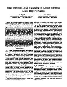
Fig 11 shows the probability of reaching the destination as a function of the threshold τ . The values are plotted for different network density. Here, L = 15, W =, Ps = 5, P¯r = 1. Clearly, the larger the τ , the smaller the probability of reaching to the destination. As ρ increases, the transition becomes sharper. When the network density is very high (ρ = 50, 100), we see an abrupt change around τ = 1.6. The critical threshold obtained from the continuum model is (π ln 2)P¯r ≈ 2.18. We expect the threshold to shift towards 2.18 as ρ increases.

Fig. 12.

1

Probability of reaching the destination at (L,0)

30

40

50

60

70

Travelling wave behavior

τ = 4 Prbar = 1 Ps = 5 d0 = 0.2

0.9

Level−1

0.8

Pk(x,0)

0.7 0.6 Level−2

0.5 0.4

1 ρ=1 ρ=5 ρ=10 ρ=50 ρ=100

0.8

20

x

Prbar = 1, L = 15, W = 2

0.9

10

Level−3

0.3 0.2 0.1

0.7

0 0

0.6

0.5

1

1.5

2

2.5

x 0.5

Fig. 13.

0.4

Transmissions die out

0.3

0.2

VI. C ONCLUSION

0.1

0

1

Fig. 11.

1.2

1.4

1.6

1.8

2

τ

2.2

2.4

2.6

2.8

In this paper, we analyzed the behavior of a wireless network with cooperative transmissions. The analysis is based on the idea of continuum approximation, which models networks with high node density. The accuracy of the continuum approximation is verified by simulations. An interesting conclusion drawn from the analysis is that there exists a phase transition in the propagation of the message as a function of node powers and the reception threshold. We believe that the techniques used in this

3

Probability of reaching the destination vs. τ

Next, we’ll consider the random channel model. We simulated the random network, and obtained the empirical density of nodes at level-k with respect to the x coordinate. This together with the continuum result Pk (x, 0) is shown for τ = 0.1 and τ = 4 in Figs. 12 9

paper can be useful in the analysis of other cooperative protocols.

It can be observed that this function is increasing. Therefore, h(·) is concave. iii) We have

VII. A PPENDIX

h(x) − h(0) h(x) = lim . x→0 x→0 x x

h0 (0) = lim

A. Proof of Lemma 1 i) First, that the function f (y) := R y+x 2let’s prove W u arctan( 2u )du is decreasing with respect to y y . The derivative of f (·) is f 0 (y) =

Apply the change of variables v = u/x to the R h(x)+x 2 1 τ integral h(x) u arctan( 2u )du = P¯ . Then r

Z

2 W 2 W arctan( )− arctan( ). y+x 2(y + x) y 2y

h(x) x

By inspection it can be seen that f 0 (y) < 0. This proves that f (·) is decreasing. Notice that f (0) = ∞ and f (∞) = 0. Thus, the equation f (y) = τ has a unique solution R h(x)+xin2 terms of 1y . τ ii) We know that h(x) u arctan( 2u )du = P¯r . By taking derivative of both sides with respect to x, we get h0 (x) =

U (h(x) + x) , U (h(x)) − U (h(x) + x)

h(x) x

+1

2 1 τ arctan( )dv = ¯ . v 2vx Pr

By taking the limit x→0, ½ ¾ Z h0 (0)+1 2 1 τ lim arctan( ) dv = ¯ . v x→0 2vx Pr h0 (0) Since limy→∞ arctan(y) = π2 , Z h0 (0)+1 π τ dv = ¯ . v Pr h0 (0)

(26)

τ

Direct evaluation gives h0 (0) = 1/(e πP¯r − 1). 1 1 iv) From (26) observe that h0 (x)→0 as x→∞. If where U (x) := x arctan( ³ 2x ). The derivative ´of 1 1 2 h0 (0) > 1, then h(x) > x for x > 0 small enough. U (·) is U 0 (x) = −1 x x arctan( 2x ) + 4x2 +1 . Since, h(·) is increasing and h0 (x)→0, h(x) < x Since U 0 (x) < 0 for x > 0, U (·) is a decreasing for x large enough. Since h is continuous, h(x) = function. This implies that h0 (x) is positive for x for some x > 0. This fixed point is unique, since x > 0. Thus, h(·) is increasing. h(·) is increasing but not linear. In order to simplify notation, we’ll use h instead of When h0 (0) < 1, h(x) < x for sufficient small h(x). Next, we will prove that h00 (x) < 0, which x > 0. It follows from the concavity that h(x) < implies the concavity of h(·). Observe x for all x > 0. Therefore, h(x) = x can only (h0 + 1)U 0 (h + x)U (h) − U (h + x)U 0 (h)h0 happen at x = 0. 00 h (x) = . (U (h) − U (h + x))2 In order to prove h00 (x) < 0, we need to show that the numerator above is negative, i.e.,

R EFERENCES [1] G. Kramer, M. Gastpar, and P. Gupta, “Cooperative strategies and capacity theorems for relay networks,” submitted to IEEE Trans. Inform. Theory, Feb. 2004. [2] A. Sendonaris, E. Erkip, and B. Aazhang, “Increasing uplink capacity via user cooperation diversity,” Proc. IEEE Int. Symp. Inform. Theory, p. 156, 1998. [3] A. Sendonaris, E. Erkip, and B. Aazhang, “User cooperation - Part I: System description,” and “User cooperation - Part II: Implementation aspects and performance analysis,” IEEE Trans. on Comm., v. 51 , no. 11, Nov. 2003. [4] J. N. Laneman and G. W. Wornell, “Distributed space-time coded protocols for exploiting cooperative diversity in wireless networks,” IEEE Trans. Inform. Theory, vol. 59, no. 10, pp. 2415-2525, Oct. 2003. [5] D. Gunduz and E. Erkip, ”Joint source-channel cooperation: Diversity versus spectral efficiency,” Proceedings of 2004 International Symposium on Information Theory, Chicago, June 2004. [6] M. Yuksel and E. Erkip, ”Diversity gains and clustering in wireless relaying,” Proceedings of 2004 International Symposium on Information Theory, Chicago, June 2004.

(h0 + 1)U 0 (h + x)U (h) < U (h + x)U 0 (h)h0 . (27)

Since h0 is positive, (27) is equivalent to h0 + 1 0 U (h + x)U (h) < U (h + x)U 0 (h). (28) h0

Substitute (26), to get is equivalent to

h0 +1 h0

=

U (h) U (h+x) .

Hence, (28)

−U 0 (h) −U 0 (h + x) > . U 2 (h + x) U 2 (h)

It suffices to show that the function l(x) := is increasing. Substitute U to get l(x) =

1 arctan( 2x )+

2x 4x2 +1

1 arctan2 ( 2x )

−U 0 (x) U 2 (x)

.

10

[7] S. Borade, L. Zheng and R. Gallager, “Maximizing degrees of freedom in wireless networks,” Proc. Allerton Conference, 2003. [8] I. Maric and R. Yates, “Efficient Multihop Broadcast for Wideband Systems, Book chapter: Multiantenna Channels: Capacity, Coding and Signal Processing”, DIMACS Workshop on Signal Processing for Wireless Transmission, Piscataway, Oct. 2002. [9] A. Scaglione and Y.-W.Hong, “Opportunistic large arrays: Cooperative transmission in wireless multihop adhoc networks to reach far distances,” IEEE Trans. on Signal Proc., vol. 51, No. 8, Aug. 2003. [10] Y.-W.Hong and A. Scaglione, “Energy-efficient broadcasting with cooperative transmission in wireless sensory ad hoc networks,” Proc. Allerton, Oct. 2003. [11] B. Sirkeci-Mergen and A. Scaglione “Coverage Analysis of Cooperative Broadcast in Wireless Networks”, Workshop on Signal Processing Advances in Wireless Communications (SPAWC), July 11-14 2004, Lisbon, Portugal. [12] B. Sirkeci-Mergen and A. Scaglione, “Signal acquisition for cooperative transmissions in multi-hop ad-hoc networks,” ICASSP 2004 . [13] B. Sirkeci-Mergen and A. Scaglione, “A continuum approach to dense wireless networks with cooperation,” Technical Report, Cornell University, School of Elec. and Comp. Eng., June 2004. [14] O. Dousse and P. Thiran, “Connectivity vs. capacity in dense ad hoc networks,” Proceedings of IEEE Infocom, Hong Kong, March 2004. [15] A. Jovicic, P. Viswanath and S. R. Kulkarni, “Upper bounds to transport capacity of wireless networks,” submitted to IEEE Trans. on Inform. Theory (revised, Mar. 2004). [16] C. Comaniciu and H.V. Poor, “On the capacity of mobile ad hoc networks with delay constraints,” IEEE Trans. on Wireless Comm., to appear. [17] D. Tse and P. Viswanath, “EECS 224B: Fundamentals of Wireless Communications,” lecture notes, University of California, Berkeley, Spring 2004. Available at http://degas.eecs.berkeley.edu/∼dtse/. [18] T. S. Rappaport, Wireless Communications Principles and Practice, Second Edition, Prentice Hall. [19] R. L. Devaney, An Introduction to Chaotic Dynamical Systems, 2nd Ed. Perseus Publishing Co., a division of Harper/Collins, 1989.

11