viability of servocontrol of pneumatic actuators via solenoid on/off valves [6-10], they have in general been marked by a lack of a rigorous analytical approach ...
Proceedings of IMECE’02 2002 ASME International Mechanical Engineering Congress & Exposition New Orleans, Louisiana, November 17-22, 2002
IMECE2002-DSC-33424 A CONTROL DESIGN METHOD FOR SWITCHING SYSTEMS WITH APPLICATION TO PNEUMATIC SERVO SYSTEMS Eric J. Barth Michael Goldfarb Department of Mechanical Engineering Vanderbilt University Nashville, TN 37235
ABSTRACT The motivation for this work is to formulate a control design method for a pneumatic system with discrete input values (resulting from the use of binary or three-position solenoid valves) that addresses the time-delay that is often associated with the flow state of solenoid on/off valves. This method is shown to be applicable to a general class of nonlinear, nonautonomous systems subject to possibly discontinuous governing dynamics. This method is then extended for timedelayed systems and applied to the case of LTI models with a finite number of allowed input values possessing a pure time delay. A pneumatic inertial positioning system employing binary solenoid valves exhibiting a time delay is modeled, and the control design method proposed is applied. An experimental implementation of the resulting control law for accurate position tracking utilizing only position feedback demonstrates the effectiveness of the method.
servovalves. Though previous research has demonstrated the viability of servocontrol of pneumatic actuators via solenoid on/off valves [6-10], they have in general been marked by a lack of a rigorous analytical approach with which to design and analyze such a system. Exceptions include the work by van Varseveld and Bone [11], Barth et. al. [12, 13] and Paul et. al. [14]. The work by van Varseveld and Bone [11] experimentally develops a discrete-time model of a PWMcontrolled pneumatic servo system with an autoregressive system identification approach, then applies discrete-time control methods to develop a controller. Barth et. al. [12, 13] provides a method to transform the non-analytic description of PWM-based control of pneumatic systems into an analytic model, which in turn enables the use of conventional analytical control approaches such as frequency domain design and sliding mode control. The work by Paul et. al. [14] formulates a controller that directly switches the valves by evaluating the derivative of the chosen Lyapnuov function. The work by Paul et. al. [14] is similar to the method presented here, in that it is a special case. The work by Paul et. al. is extended here to include a control design method for a more general class of system models including nonlinear, non-autonomous switching models which need not be affine in the control variable, as well as for the case of time-delayed LTI systems. Paul et. al. showed experimental results for position step commands, whereas sinusoidal tracking is demonstrated here.
1. INTRODUCTION Servo control of pneumatic systems is generally implemented via the proportional control of servovalves, in which pneumatic fluid flow is controlled via proportional constriction (i.e., throttling). This proportional control approach has been studied by several researchers, including Shearer [1], Liu and Bobrow [2], Kunt and Singh [3], Ye et al. [4], and Bobrow and McDonell [5]. The control of such systems is complicated by the need to accurately describe the flow characteristics of a proportional servovalve, which is typically accomplished empirically with a set of pressure/flow relationships.
The motivation for this work is to formulate a control design method for a pneumatic system with discrete input values (resulting from the use of binary or three-position solenoid valves) that addresses the time-delay that is often associated with the flow state of solenoid on/off valves. The resulting control design method, as applied to pneumatic systems, avoids the use of costly proportional servovalves and
Switching control, via binary-position solenoid valves, offers an alternative to the servovalve control approach that both circumvents the accurate dynamic characterization of throttling a fluid flow, and avoids the high cost of proportional
1
Copyright © 2002 by ASME
upon the selection of the input, and a measurable non-candidate term independent of the input:
pressure sensors (the two most expensive components of a pneumatic servo system) while achieving accurate tracking. Though this work is motivated by pneumatic servo control, a general control design methodology for switching systems with a finite set of discrete input values is presented that provides a stability guarantee. This control design method is applicable to general nonlinear, non-autonomous, discontinuous system models (as a result of potentially both discontinuous finite valued inputs, as well as discontinuous finite valued governing dynamics) that have no time-delay associated with the control variables. Based on this, a control design method is then presented for LTI models that have a finite set of allowable control inputs with a pure time delay. Although not presented here, the method for LTI switching systems with time delay can be extended to the more general case of nonlinear, nonautonomous, discontinuous system models with a time delay by using an appropriate nonlinear model-based predictor. To illustrate the control design method, the tracking control of single degree-of-freedom pneumatic inertial positioning system is formulated and experimentally implemented.
n æ n ö d n-r dn s& = b(x)u + f (x) - n xd + å çç ÷÷lr n-r e 123 dt dt 1 èrø candidate term 144444 42r =4 44444 3 non -candidate term
If the input to the plant is only allowed to be a finite set of p discrete values, u Î {u1 , u2 , K , u p }
where the state vector is x = [ x, x&, K , x T
V&i = s (e ( n -1) ,K, e) s&(ui , x, xd( n ) , e ( n -1) ,K, e) for i = {1,2,K, p}
i
values, each V&i term can be computed on-line in real-time and u may be selected according to the following control law: j ={1, 2 ,K, p}
] , and the
1 2 s 2
for i = {1,2,K, p}
n
n -1 n æ ö r d n-r -1 n çç ÷÷l n-r -1 e = l + edt edt å ò ò dt r =0 è r ø
(2)
(3)
where e = x - xd . Note that s is a measurable quantity if di xd for i = {0, 1, K , n} is known. Stability in the Lyapunov dt i sense is guaranteed and the error is driven to zero when the following condition is enforced: V& = ss& £ 0
(8)
That is, the ui corresponding to the least negative V&i is selected. In one sense, this control law can be viewed as traditional sliding mode control without the equivalent control term. In a more general sense, it is a method that directly enforces the stability and error convergence condition by selecting trial inputs and evaluating the expected V& . In this sense, as will be seen below, the method is applicable to more general dynamic systems which are not affine in the control variable due to the fact that the control is not being “solved for”. Implementation of such a control law would most likely be impractical for systems of order greater than three due to measurement noise associated with the higher derivative terms contained in Equation (7). That being said, most pneumatic systems can be adequately modeled with a third order system, and therefore avail themselves to such a control technique (if being controlled by discrete-position valves).
Choose the typical integral sliding surface as, æd ö s = ç + l÷ è dt ø
( )
u = u i such that V&i = max V& j and V&i £ 0
exponent term enclosed in parentheses · (n ) is a shorthand notation for the nth derivative with respect to time. Define the following continuous positive definite Lyapunov function: V=
(7)
The stability and error convergence condition given by Equation (4) may be enforced by selecting an input value ui with an associated V& £ 0 . Given a finite set of allowable input
(1) ( n -1)
(6)
each input value ui will have an associated V&i term:
2. CONTROL DESIGN FOR SWITCHING SYSTEMS Assume the plant dynamics are given in the following form,
dn x = f (x) + b(x)u dt n
(5)
The method presented above can be further generalized whereby multiple valves with multiple discrete positions may be incorporated into the control law. This can be accomplished by forming all possible permutations of the discrete positions of the valves and assigning each permutation a candidate term V&i ,
(4)
Substituting in the plant dynamics, Equation (1), s& may be expressed as the summation of a candidate term dependent
2
Copyright © 2002 by ASME
as dictated by the plant dynamics corresponding to those valve positions. The selection of a correct permutation of discrete input values is then provided by extending the control law given by Equation (8) to the multiple input case. In the case where the plant dynamics are different for each permutation, the plant can more generally be given by, dn x = f i (x, u) , "u Î {u i : i = 1,2, K , p} dt n
dn x(t ) = f i (x(t ), u(t - TD ) ) , "u Î {u i : i = 1,2, K , p} (9) dt n where TD is the pure delay in the system. The estimated derivative of the Lyapunov function can be put in the following form,
& Vˆi (t + TD ) = sˆ(t + TD ) s&ˆ(t , t + TD )
(1a)
where s& is then given more generally as: s& = f i (x, u) -
n æ n ö d n- r dn x + å çç ÷÷lr n-r e n d dt dt r =1 è r ø
where estimates sˆ and s&ˆ are given more explicitly as:
(
sˆ(t + TD ) = sˆ eˆ ( n-1) (t + TD ), K , eˆ(t + TD )
(5a)
(
(6a)
for i = {1,2,K, p}
(7a)
( )
j ={1, 2 ,K, p}
for i = {1,2,K, p}
)
(12)
Although estimates of future states may be made for the general nonlinear system(s) of Equation (9), consider here the SISO case where the system dynamics are given by the following LTI model:
The control u may be selected according to the control law: u = u i such that V&i = max V& j and V&i £ 0
(11)
Therefore, in order to select the current input u(t ) at time t & that will result in Vˆi (t + TD ) £ 0 at the future time t + TD , it is necessary to estimate the future states xˆ (t + TD ) , and necessary to have available the future desired states x d (t + TD ) .
Each input vector u i has an associated V&i term: V&i = s (e ( n -1) ,K , e) s&(u i , x, xd( n ) , e ( n -1) ,K, e)
)
s&ˆ(t , t + TD ) = s&ˆ u i (t ), xˆ (t + TD ), x d( n ) (t + TD ), eˆ ( n-1) (t + TD ),K, eˆ(t + TD )
The permutations of the discrete-valued multiple inputs form the following set, of which the selected input is a member: u Î {u1 , u 2 , K , u p }
(10)
(8a)
x& (t ) = Ax(t ) + Bu(t - TD )
(13)
To obtain a model-based prediction of future states xˆ (t + TD ) starting from the present measurable state x(t ) , the timedomain solution of Equation (13) with an initial condition x(t ) can be written as:
The dynamic system given by Equation (1a) is a switching system not only in the sense that the inputs may switch discontinuously between discrete values, but also that the system dynamics f i (x, u) may switch discontinuously as well. Also note that although x (n ) is discontinuous, it is assumed to be finite thereby making x and therefore V continuous, as required for the stability analysis.
xˆ (t + TD ) = e AT x(t ) +
t +TD
òe
D
0
t
- òe
3. CONTROL DESIGN FOR LTI SWITCHING SYSTEMS WITH TIME DELAY For pneumatic systems whereby control is achieved with discrete position valves (such as binary or three-position, threeway solenoid valves), a time delay in the response of the valve is often observed as an inherent property of the configuration of such valves. To apply the above control design procedure to systems with a pure time delay, a model-based predictor is required to estimate future values of V&i for the selection of the present input value. Consider a dynamic system of the form,
A (t - t)
A (t - t)
Bu(t - TD )dt (14)
Bu(t - TD )dt
0
It is important to note that the prediction given by Equation (14) involves only past values of the input, measurable quantities x(t ) , and e AT which can be computed off-line for a known time delay. The present control u(t ) is selected by Equations (10-12), Equation (14), and the following control law: D
3
Copyright © 2002 by ASME
gm& RT - gPV& P& = V
u(t ) = u i (t) & & such that Vˆi (t + TD ) = max æçVˆ j (t + TD ) ö÷ j ={1, 2 ,K, p}è ø &ˆ and Vi (t + TD ) £ 0 for i = {1,2, K , p}
(15)
where g is the ratio of specific heats. A more general polytropic model is also of the form of Equation (17) where g becomes the polytropic exponent. Pursuant to modeling a switching system, it will only be necessary to model the pressure dynamics of each chamber in response to connecting the chamber to either the high-pressure supply or exhausting it to atmosphere. These valving operations are reflected in the mass flow rate term m& of Equation (17). The mass flow of a gas is often modeled as two flow regimes dependent on the upstream and downstream pressures. Denoting Phigh and Plow as the upstream and downstream pressures respectively, subsonic and supersonic (choked) flow conditions result in the following commonly accepted models (stated for air):
Although not presented here, the above method for LTI switching systems with time delay can be extended to the more general case of nonlinear, non-autonomous, discontinuous system models (Equation (9)) with time delay by using an appropriate nonlinear model-based predictor. 4. MODELING A PNEUMATIC POSITIONING SYSTEM CONTROLLED VIA SWITCHING VALVES Consider the single degree-of-freedom pneumatic actuation system shown in Figure 1. This inertial positioning system with discrete input values will be used to exemplify the control design procedure proposed. A lumped-parameter model that treats all unmodeled forces, such as coulomb and viscous friction and external disturbance forces, as a single disturbance term is given as,
M &x& = PB AB - PA AA + Fdisturbance
1/ 2
æ 2 ö ÷ [ Plow ( Phigh - Plow )]1 / 2 m& = cA0 eç ç RThigh ÷ è ø for Phigh < 1.89 Plow
(16)
where PA and PB are the pressures (gage) inside chambers A and B of the pneumatic actuator respectively and AA and AB are the areas of the piston seen by each chamber. The pressure in each chamber will be controlled by a two-position valve that serves to connect the chamber to either a high pressure supply or to atmospheric pressure.
P E P E
P = Supply Pressure E = Exhaust
Chamber B
1/ 2
æ 1 ö é æ 2 ö ( g +1) /( g -1) ù ÷ ê gç ÷ ú m& = cA0 Phigh ç ç RThigh ÷ ê çè g + 1 ÷ø úû è ø ë for Phigh > 1.89 Plow
(18a)
1/ 2
(18b)
Since the orifice size A0 is dependent on the dynamics of the valve opening or closing and the discharge coefficient c must be measured experimentally, Equations (18a, 18b) are in practice difficult to use. Additionally, including the dynamics of A0 would undesirably increase the order of the model.
P E P E
Chamber A
(17)
To obtain a reduced order model of the mass flow, there are certain features that can be exploited by operating the valves in a switching mode. The first feature that can be taken advantage of is that the orifice size A0 , or rather the dynamics of the orifice size, can be assumed to be independent of operating conditions. This is reflective of two assumptions: 1) in a switching mode of operation the valve is always being commanded to be completely opened or completely closed, and 2) the impedance of the valve’s response is high (i.e. the opening and closing response of the valve is not appreciably influenced by the pressures on either side of the valve for the pressure ranges of interest). A second feature that simplifies the modeling is that the driving pressure is either the supply pressure or atmospheric pressure. Assuming that these pressures are constant, these then become merely parameters of the model. Therefore, for repeatable valve operation and
M x
FIGURE 1. SCHEMATIC DIAGRAM OF A PNEUMATIC INERTIAL POSITIONING SYSTEM ACTUATED WITH A DOUBLE-ACTING PNEUMATIC CYLINDER AND CONTROLLED WITH TWO BINARY (2-POSITION) 3-WAY PILOT-ASSISTED SOLENOID VALVES.
From an energy balance, the pressure in a chamber of variable volume influenced by a mass flow rate into or out of the chamber can be modeled as the following, assuming an adiabatic and reversible process (isentropic) involving an ideal gas,
4
Copyright © 2002 by ASME
conditions of fixed supply and atmospheric pressures and external temperature, the term gm& RT / V of Equation (17) is a function solely of chamber pressure, chamber volume and a discrete-valued input term of either supply or exhaust pressure. As a result, Equation (17) can be approximately modeled for each chamber as, ( P + Patm ) gAA, B x& u - PA, B P&A, B = A, B ± A, B c A, B m AA, B x t A, B ( x , u A , B )
above, the plant model for the pneumatic system under consideration here can be written as,
[
]
1 Psupply u (t - TD ) - M &x&(t ) , Mt "u Î {u i : i = 1,2,3}
&x&&(t ) =
where:
(19)
u1 = - AA ,
where t A, B is shown as an explicit function of the input
u2 = 0 ,
u3 = AB
(22)
The control design procedure for time-delayed LTI switching systems given by Equations (10-15) is now applicable to the pneumatic switching system described by Equations (21, 22).
pressure u A, B (supply pressure or atmospheric pressure) and piston position x (linearly proportional to chamber volume V). Implicit is the functional dependence on those parametric variables mentioned above. The constants c A, B represent the volumes of the chambers at the midpoint position of the actuator ( x = 0 ). Assume that the first term of Equation (19) may be modeled sufficiently accurately with a constant value for t A, B . Further assume that for typical pneumatic actuators operated with typical supply pressures, the second term of Equation (19) can be neglected. The pressure dynamics may therefore be approximated by the following linear model: u - PA, B P&A, B = A, B t A, B
(21)
5. EXPERIMENTAL RESULTS The preceding analysis and control approach was experimentally implemented on a single degree-of-freedom pneumatically actuated servo system as shown in Figure 1. This setup included a 1.905 cm (3/4 inch) inner diameter, 10 cm (3.9 inch) stroke double-acting pneumatic cylinder (Bimba 044-DXP) equipped with two pilot-assisted, binary, 3-way, solenoid-activated valves (SMC VQ1200H-5B), a 10 kg brass block on a track with linear bearings (Thompson 1CBO8FAOL10), a linear potentiometer (Midori LP-100F) for position feedback, and three pressure transducers (Omega PX202) for model validation and to monitor the pressures, but not used for control. Model parameters were estimated or measured to be: M = 10 kg, AA = 2.5 cm 2 , AB = 2.8 cm 2 , c A =
(20)
The model given by Equation (20) can be experimentally determined for a particular valve and a particular pneumatic actuator. Specifically, t A, B can be estimated from data by matching the modeled and measured dynamic pressure response of each chamber of the actuator as it is pressurized and exhausted at the midpoint piston position.
12.6 cm 3 , c B = 14.2 cm 3 , g = 1.4 and a supply pressure of 586 kPA (85 psig). For the system and components experimentally implemented here, the value of t in Equations (20, 21) and the time delay TD in Equation (21) was estimated from data by matching the modeled and measured pressure dynamics of each chamber of the actuator as it was pressurized and exhausted while held at the midpoint piston position x = 0.0 cm . Figure 2 compares the results of this modeling to the measured response. This resulted in estimated values of t = t A = t B = 11
To model the effects of the two valves operating in a switching mode, all permutations of the discrete inputs to the two valves must be enumerated. The permutations, or modes, of operation are the following (in gage pressures): Mode 1: u A = Psupply and u B = 0
ms and TD = 20 ms. The values of t and TD were selected in conjunction, rather than individually, so that the modeled response gave a good overall match to the measured response.
Mode 2: u A = 0 and u B = 0 Mode 3: u A = 0 and u B = Psupply Mode 4: u A = Psupply and u B = Psupply
The control law implemented was that given by Equation & (15) where each Vˆ (t + T ) was evaluated according to
For the particular system being exemplified here, it will be assumed that Mode 4 is not used since it seems to have little utility with regard to this system. Given that the valve has some time delay TD associated with its response, and given Equation (16), Equation (20), and Modes 1, 2, and 3 as listed
i
D
Equations (10), (11), and (12), with xˆ (t + TD ) estimated in realtime by Equation (14) and the state-space representation of the system model given by Equation (21). If at any point in time a control input satisfying the control law did not exist due to
5
Copyright © 2002 by ASME
Chamber B 90
80
80
70
70
60
60 Pressure (psig)
Pressure (psig)
Chamber A 90
50 40
50 40
30
30
20
20
10
10
0
0
0.05
0.1 0.15 Time (sec)
0.2
0
0.25
0
0.05
0.1 0.15 Time (sec)
0.2
0.25
FIGURE 2. DATA USED TO EMPIRICALLY OBTAIN t = 11 MS AND TD = 20 MS. SHOWN ABOVE IS THE MEASURED PRESSURE RESPONSE (SOLID LINE) AND MODELED RESPONSE (DASHED LINE)
Mass position (cm)
0.5 Hz
1 Hz
3
3
2
2
1
1
0
0
-1
-1
-2
-2
-3
0
0.5
1
1.5
2
2.5
-3
3
0
0.5
1
Mass position (cm)
2 Hz 3
2
2
1
1
0
0
-1
-1
-2
-2
0
0.5
1
1.5 Time (sec)
2
2.5
3
2
2.5
3
3 Hz
3
-3
1.5
2
2.5
-3
3
0
0.5
1
1.5 Time (sec)
FIGURE 3. EXPERIMENTAL CLOSED-LOOP TRACKING OF THE LOAD MASS POSITION AT 0.5 HZ, 1 HZ, 2 HZ, AND 3 HZ. THE COMMANDED POSITION IS SHOWN AS DASHED AND THE MEASURED POSITION IS SHOWN AS SOLID.
6
Copyright © 2002 by ASME
modeling errors and/or noise, the control input with the & smallest positive associated Vˆi (t + TD ) term was selected. The integral sliding surface was selected as Equation (3) using a value of l = 20 × 2p . A differentiating filter was selected to be of the form, D(s) =
s a 2 s 2 + 2as + 1
[5] Bobrow, J., and McDonell, B., 1998, “Modeling, Identification, and Control of a Pneumatically Actuated, Force Controllable Robot,” IEEE Transactions on Robotics and Automation, vol. 14, no. 5, pp. 732-742. [6] Morita, Y. S., Shimizu, M., and Kagawa, T., 1985, “An Analysis of Pneumatic PWM and its Application to a Manipulator,” Proc. of International Symposium of Fluid Control and Measurement, Tokyo, pp. 3-8.
(23)
with an 80 Hz cutoff frequency to obtain the signals x& , &x& , x& d , &x&d , &x&&d from x and xd . The tracking performance for this controller is shown in Figure 3 for 0.5, 1, 2, and 3 Hz.
[7] Noritsugu, T., 1985, “Pulse-Width Modulated Feedback Force Control of a Pneumatically Powered Robot Hand,” Proc. of International Symposium of Fluid Control and Measurement, Tokyo, pp. 47-52.
6. CONCLUSIONS A method was presented for the control design of switching systems with a finite number of discrete input values. This included general nonlinear, non-autonomous system models with discontinuous governing dynamics without time delay, as well as LTI systems with time delay. The method provides a direct evaluation of the stability and error convergence condition and thereby offers both stability and tracking guarantees. Furthermore, since this method directly evaluates each control candidate, it does not require obtaining a closedform expression for the control law and is therefore applicable to a very general class of dynamic systems. The proposed control design method for time-delayed LTI switching systems was applied experimentally to a pneumatic inertial positioning system controlled with pilot-assisted solenoid valves. The resulting control law required only position feedback information (i.e. no pressure sensors were required). Sinusoidal tracking of this system demonstrated the effectiveness and simplicity of the control design method.
[8] Noritsugu, T., 1986, “Development of PWM Mode Electro-Pneumatic Servomechanism. Part I: Speed Control of a Pneumatic Cylinder,” Journal of Fluid Control, vol. 17, no. 1, pp. 65-80. [9] Noritsugu, T., 1986, “Development of PWM Mode Electro-Pneumatic Servomechanism. Part II: Position Control of a Pneumatic Cylinder,” Journal of Fluid Control, vol. 17, no. 2, pp. 7-31. [10] Lai, J.-Y., Singh, R., and Menq, C.-H., 1992, “Development of PWM Mode Position Control for a Pneumatic Servo System,” Journal of the Chinese Society of Mechanical Engineers, vol. 13, no. 1, pp. 86-95. [11] van Varseveld, R. B., and Bone, G. M., 1997, “Accurate Position Control of a Pneumatic Actuator Using On/Off Solenoid Valves,” IEEE/ASME Transactions on Mechatronics, vol. 2, no. 3, pp. 195-204.
REFERENCES [1] Shearer, J. L., 1956, “Study of Pneumatic Processes in the Continuous Control of Motion With Compressed Air – I,” Transactions of the ASME, February, pp. 233-242.
[12] Barth, E. J., Zhang, J., and Goldfarb, M., 2001, “A Method for the Frequency Domain Design of PWM-Controlled Pneumatic Systems”. Proceedings of IMECE2001, Volume 2: 2001 ASME International Mechanical Engineering Congress and Exposition (IMECE), November 11-16.
[2] Liu, S., and Bobrow, J. E., 1988, “An Analysis of a Pneumatic Servo System and Its Application to a ComputerControlled Robot,” ASME Journal of Dynamic Systems, Measurement, and Control, vol. 110, no. 3, pp. 228-235.
[13] Barth, E. J., Zhang, J., and Goldfarb, M., 2002, “Sliding Mode Approach to PWM-Controlled Pneumatic Systems”. 2002 American Control Conference (ACC), in press.
[3] Kunt, C., and Singh, R., 1990, “A Linear Time Varying Model for On-Off Valve Controlled Pneumatic Actuators,” ASME Journal of Dynamic Systems, Measurement, and Control, vol. 112, no. 4, pp. 740-747.
[14] Paul, A. K., Mishra, J. K., Radke, M. G., 1994, “Reduced Order Sliding Mode Control for Pneumatic Actuator,” IEEE Transactions on Control Systems Technology, vol. 2, no. 3, pp. 271-276.
[4] Ye, N., Scavarda, S., Betemps, M., and Jutard, A., 1992, “Models of a Pneumatic PWM Solenoid Valve for Engineering Applications,” ASME Journal of Dynamic Systems, Measurement, and Control, vol. 114, no. 4, pp. 680-688.
7
Copyright © 2002 by ASME