A cutting-plane method for contiguity-constrained spatial aggregation

J OURNAL OF S PATIAL I NFORMATION S CIENCE Number 15 (2017), pp. 89–120

doi:10.5311/JOSIS.2017.15.379

R ESEARCH A RTICLE

A cutting-plane method for contiguity-constrained spatial aggregation Johannes Oehrlein and Jan-Henrik Haunert Institute of Geodesy and Geoinformation, University of Bonn, Germany

Received: September 11, 2016; returned: November 17, 2017; revised: November 26, 2017; accepted: November 28, 2017.

Abstract: Aggregating areas into larger regions is a common problem in spatial planning, geographic information science, and cartography. The aim can be to group administrative areal units into electoral districts or sales territories, in which case the problem is known as districting. In other cases, area aggregation is seen as a generalization or visualization task, which aims to reveal spatial patterns in geographic data. Despite these different motivations, the heart of the problem is the same: given a planar partition, one wants to aggregate several elements of this partition to regions. These often must have or exceed a particular size, be homogeneous with respect to some attribute, contiguous, and geometrically compact. Even simple problem variants are known to be NP-hard, meaning that there is no reasonable hope for an efficient exact algorithm. Nevertheless, the problem has been attacked with heuristic and exact methods. In this article we present a new exact method for area aggregation and compare it with a state-of-the-art method for the same problem. Our method results in a substantial decrease of the running time and, in particular, allowed us to solve certain instances that the existing method could not solve within five days. Both our new method and the existing method use integer linear programming, which allows existing problem solvers to be applied. Other than the existing method, however, our method employs a cutting-plane method, which is an advanced constraint-handling approach. We discuss this approach in detail and present its application to the aggregation of areas in choropleth maps. Keywords: area aggregation, districting, spatial unit allocation, optimization, integer linear programming, cutting-plane method, map generalization, choropleth map

c by the author(s)

CC Licensed under Creative Commons Attribution 3.0 License

90

1

O EHRLEIN , H AUNERT

Introduction

Planar subdivisions are frequently used to structure geographic space. In geographic information systems, they can be used as a basis for data acquisition, storage, analysis, and visualization. Since different applications require information on different scales, planar subdivisions are often hierarchical—unemployment rates, for example, can be analyzed on a county or country level. Often, one aims to compute a higher-level subdivision from a given one, by grouping areas of similar attribute values. With such an approach, one can reveal large-scale patterns in the data. In this article, we present a new method for area aggregation, which we discuss in the context of districting and spatial unit allocation. We distinguish these problems as follows: • Districting [9, 36, 38, 62] is the problem of partitioning a set of minimum mapping units (e.g., postal code zones) to form larger regions or districts (e.g., school zones or electoral districts). The minimum mapping units (i.e., input areas) are assumed to form a planar subdivision. The applications of districting range from administrative to commercial purposes; an overview is provided by Shirabe [61]. • Spatial unit allocation [60, 61] subsumes districting, but it does not necessarily ask to assign every area to a district. A typical example of spatial unit allocation is to select a set of areas constituting a single region that is geometrically compact and requires minimal development costs [1]. • The term area aggregation has been used to refer to the aggregation of areas as a data abstraction or map generalization problem [34]. Just as districting, area aggregation requires a planar subdivision as input and asks to group the areas into larger regions. Districting problems in spatial planning, however, do not necessarily ask to group areas of similar attribute values, which is an essential criterion for generalization. It is common to approach districting, spatial unit allocation, and area aggregation by optimization [7, 20, 29, 33, 45, 49, 62]. The existing approaches are quite similar, since the different problem variants often share some optimization objectives and constraints. For example, it is common to require that every output region must have a size or population within certain bounds and to favor geometrically compact shapes. Compactness is usually assessed quantitatively, which can be done with different measures [44,47], and considered as an optimization objective. Additionally, in many problem variants, the output regions are required to be contiguous [14, 20, 61, 62, 69]: Definition 1. An area A ⊆ R2 is called contiguous if every two points in A are connected via a (not necessarily straight) line that is contained in A. Though the output regions tend to become contiguous when compactness is considered as an objective, there is generally no guarantee for contiguity without enforcing it. In fact, if compactness is not the primary objective, contiguity often has to be enforced to produce somehow reasonable output regions [62]. Therefore, we think that optimizing similarity (and compactness as a secondary criterion) subject to size constraints and contiguity is a particularly interesting challenge. Attribute similarity is an important criterion for aggregation in map generalization, which means to generate a more abstract and less detailed representation of geographic space from a given one [8, 59, 68]. The problem occurs if the scale of a cartographic visualization has to be reduced, but map generalization does not necessarily assume that the input www.josis.org

A C UTTING -P LANE M ETHOD FOR C ONTIGUITY-C ONSTRAINED S PATIAL AGGREGATION

v1

v2 v4

v7

v3 v5

v8

91

v6

v9

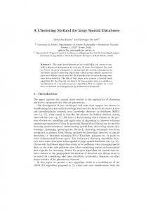
(a) Explanatory maps: input map (left) and output map (right).

(b) The adjacency graph G = (V, E) for the input map in (a) and the partition of V corresponding to the output map.

Figure 1: An example of area aggregation (see Haunert and Wolff [34]).

and output representations are visual graphics. Haunert and Wolff [34] have defined the area aggregation problem in map generalization formally and developed an optimization method for it, which is based on models for districting by Zoltners and Sinha [70] and Shirabe [62]. The problem not only requires to group the input areas into larger regions, but also to assign a value from the attribute domain to each output region; see Figure 1(a). The aim is to minimize a cost function that penalizes changes of attribute values to dissimilar values as well as geometrically non-compact output regions, subject to constraints concerning the size and contiguity of the output regions. The method relies on the definition of the adjacency graph G = (V, E) whose vertex set V contains a vertex for each input area and whose edge set E contains an edge {u, v} for each two adjacent areas u, v ∈ V ; see Figure 1(b). We will use this definition of G throughout this article. In this article, we revisit the problem defined by Haunert and Wolff [34], but we also consider the special case that similarity is neglected and compactness is the sole objective. In this case, the problem is more similar to a classical districting problem that simply demands geometrically compact and contiguous regions of sizes within certain bounds. Moreover, while Haunert and Wolff developed and tested their method for the generalization of categorical maps, we will use our method to generalize choropleth maps with a ratio-scaled variable, such as unemployment rates. This has the advantage that we can directly compute differences between attribute values and do not depend on the definition of a semantic distance between categories. We focus on exact optimization methods based on integer linear programming, which is a common optimization approach for districting [9, 33, 36]. In particular, it is reasonable for NP-hard problems, for which the existence of an efficient and exact algorithm is extremely unlikely [28]. In fact, area aggregation falls into the class of NP-hard problems [34], and so do many problem variants of districting [2, 38, 57]. Defining an integer linear program (ILP) means setting up a linear program (LP) completed with an integrality constraint. While the LP defines a linear objective function and a set of linear inequality constraints over a set of variables, the integrality constraint requires that the variables receive integer values. An ILP is solved optimally if a variable assignment is found which optimizes the objective function without violating any constraint. Commonly, the LP corresponding to an ILP without integrality constraints is referred to as the LP relaxation of the ILP [52]. An illustrative example for both an LP and an ILP can be found in Figure 2. JOSIS, Number 15 (2017), pp. 89–120

92


x2

x2

x2

1

1

1

1

x1

(a) The red line marks (x1 , x2 )-values with equal objective value.

1

x1

(b) A solution to the linear program.

1

x1

(c) A solution to the integer linear program. The LP in (b) is completed with x1 , x2 ∈ Z.

Figure 2: A linear program with variables x1 and x2 ; objective is to maximize 6x1 + x2 with respect to x1 ≥ 0, x2 ≥ 0, 2x2 ≤ 7, 2x1 +4x2 ≤ 18 and x1 ≤ 4. The solution space, i.e., all pairs (x1 , x2 ) for which every given inequality is true, is marked as a blue polytope. The gray arrows in the background indicate the objective. They are orthogonal to the line of equal objective values in (a).

Whereas efficient algorithms for linear programming exist, integer linear programming is NP-hard [13, 28]. Nevertheless, an approach based on integer linear programming is promising as it allows sophisticated optimization software (e.g., CPLEX [15] and Gurobi [31]) to be applied. Even though the exact methods for solving ILPs have an exponential worst-case running time, they can be relatively fast when applied to real-world instances. Moreover, solutions of an exact method can be used as quality benchmarks to evaluate the results of (faster) heuristic algorithms. Heuristic methods for districting have been developed by several researchers [7, 19, 37, 43, 50]. In contrast to exact methods, these do not guarantee to deliver an optimal solution. Just as some criteria are shared by many problem variants of districting and spatial unit allocation, the ILP formulations for these problems often share some elementary components. Shirabe [63] has used this fact to integrate mathematical programming techniques and geographic information systems (GIS), such that a GIS user can assemble a model for a particular spatial unit allocation problem from a set of elementary model components and compute a solution to the problem with an ILP solver. Since contiguity is an important requirement in many spatial unit allocation problems, several works have focused on formalizing contiguity as one such elementary model component [61, 62, 69]. Usually, there exist multiple possibilities of encoding a particular problem as an ILP; choosing among these ILP formulations can highly influence the computation time. In geographic information (GI) science, it is common to choose a compact ILP formulation, which means that the size of the ILP is polynomial in the size of the input [24]. For example, in Section 2.2 we show that, when applying Shirabe’s model [61] to area aggregation without prescribing the number of output regions, it has O(n2 ) variables and constraints (where n is the number of input areas) and thus a polynomial size. A compact ILP formulation can be favorable because it permits a full instantiation of the model, that is, a file or data structure explicitly storing all variables and constraints. After the instantiation of the model, it can www.josis.org


93

be handed over to a solver, which computes an optimal solution without requiring any further interaction. It is therefore common to think of the solver as a black box [46]. Working with compact ILP formulations is relatively convenient. It is also known, however, that they are sometimes outperformed by non-compact ILP formulations, whose number of constraints can be exponential in the size of the input [56]. Such a large set of constraints forbids a full instantiation of the model. Therefore, one starts the computation by working with a reduced ILP, which is lacking a set of constraints of the original ILP. A simple approach is to solve this reduced ILP to optimality and to examine whether the solution violates constraints of the original ILP. If a violation of a constraint is found, that constraint is added to the ILP and the solution process is started anew. Drexl and Haase [18] and Duque et al. [20] use this approach to solve districting problems. In particular, Duque et al. deal with the p-regions problem, in which, other than in our problem, the number p of output regions is prescribed. In this article, we present a more sophisticated approach for area aggregation. We demonstrate the effectiveness of a cutting-plane method, which generally refers to a method that adds constraints during optimization without relying on an optimal solution to the reduced ILP. Violated constraints are found already in a preliminary stage of a solution, namely in an optimal solution to the LP relaxation of the reduced ILP. Such constraints are termed cutting planes (or simply cuts) because they cut away parts of the feasible region of the solution space defined by the current instantiation of the model. The number of constraints of our ILP formulation for area aggregation is exponential in the number n of input areas, but initially we instantiate the model with only O(n2 ) constraints. We generate constraints ensuring contiguity during optimization, using what is generally termed a separation algorithm [52]. Though implementing a cutting-plane approach requires some understanding of how an ILP solver works and certainly more effort than using a compact ILP formulation and a black-box solver, we consider it practicable, also for researchers in GI science. This is because modern ILP solvers such as CPLEX or Gurobi offer programming libraries that include interfaces (usually termed callbacks) for intervening in the optimization process. Carvajal et al. [10] have developed a cutting-plane method based on an efficient separation algorithm for a problem of spatial unit allocation in forest management. We are not aware of such a method for area aggregation or districting, though. We used the cutting plane method for contiguity-constrained spatial unit allocation by Carvajal et al. as a starting point, which, compared to the method of Drexl and Haase [18], is more recent and can be considered more sophisticated. However, we had to extend the method substantially for the case of an unknown number of output regions and a flexible set of centers. More precisely, Carvajal et al. consider two constraint formulations for the contiguity of a region, namely one that does not rely on the concept of a center of a region and one that requires a prescribed center to belong to the output region. While in the first model, contiguity is ensured by considering a set of constraints for each pair of nodes that are selected for the output region, in the second model, a set of constraints for each selected node ensures its connectivity to the prescribed center. Conceptually, our approach is more similar to the second model, as it also relies on the idea of centers. However, we do not know in advance which of the nodes become centers. Therefore, we use a constraint formulation that, in fact, is more similar to the first model of Carvajal et al. in the sense that it uses one set of constraints for each pair of nodes. Álvarez-Miranda et al. [3] and, recently, Wang et al. [66] have presented theoretical findings on integer programming formulations for the problem of selecting a maximum-weight

JOSIS, Number 15 (2017), pp. 89–120

94


connected subgraph of a given graph. Though their results cannot easily be transferred to other problems, they can be understood as hints on why a non-compact ILP formulation, such as the one of Carvajal et al. or ours, can outperform a compact ILP formulation. To summarize our contribution, we discuss cutting-plane methods as a general constraint-handling technique that is rather unknown in GI science but well established in the field of combinatorial optimization [39, 65]. We show that our cutting-plane method outperforms the districting method of Shirabe [62] that was adapted by Haunert and Wolff [34] for the aggregation of areas in map generalization. For example, with our method we were able to solve various instances with 94 departments of France (excluding overseas department and the island of Corsica) in reasonable time, whereas using Shirabe’s method produces a result in much longer time or not at all (see Section 5). We specifically apply this to generate a map that shows a structuring of France into a few (e.g., 10) regions of similar unemployment rates and thereby highlight the usefulness of the method for the generalization of choropleth maps. We do note that the applicability of our method is limited, since we were not able to process instances larger than our instances of France. The number of areas in these instances of France, however, can be considered typical for choropleth maps. Similar maps can be found, for example, in Bertin’s fundamental textbook on visualization [6]. In the following, we review an existing ILP formulation for area aggregation (Section 2). Then, we give an overview of strategies for handling ILPs with large sets of constraints (Section 3). Subsequently (Section 4), we contribute an ILP applying cutting planes which extends the ILP formulation from Section 2. Afterwards, we let both models compete in a series of experiments (Section 5). We apply both ILP formulations on a real-world example with 94 input areas, discuss the solutions, and compare the running times for different settings. We finish this article with concluding remarks and ideas for further improvements (Section 6).

2

A state-of-the-art model

The huge amount of work on spatial unit allocation and districting disallows a comprehensive review in this article. Therefore, we refer to the survey by Ricca et al. [58] for an overview and discuss only the most relevant related work that has inspired our models. This in particular concerns a general districting model with assignments of areas to centers (Section 2.1) and a flow-based model to ensure contiguous output regions (Section 2.2). In Section 2.3, we briefly review the approach of Haunert and Wolff [34] for the aggregation of areas in map generalization, which is based on the models from Sections 2.1 and 2.2.

2.1

A compact ILP without contiguity

The ILPs that we use in this article differ only with respect to the constraints ensuring contiguity. If we drop those constraints, we obtain an ILP that has the same structure as the basic ILP defined by Haunert [33]. This basic ILP follows the approach of Zoltners [70] for districting, in the sense that in every output region one of the input areas is selected as the region’s center. To encode this idea, the basic ILP uses a variable xc,v for each pair of areas www.josis.org


95

c, v ∈ V , which has the following meaning. ( 1, if area v is assigned to the output region with center c, xc,v = 0, otherwise. For c = v, the variable xc,c expresses whether area c is assigned to itself, meaning whether or not it is selected as a center. Note that with this model we do not prescribe the centers before computing an optimal assignment. Instead, every area can become a center. Each variable xc,v is associated with an assignment cost ac,v . The objective function is a weighted sum of the variables. X X min ac,v · xc,v (1) c∈V v∈V \{c}

The aim for compact output regions, for example, can be expressed by minimizing this objective function with ac,v = w(v) · d(c, v), where w(v) is a weight for area v (reflecting size or population) and d(c, v) is the Euclidean distance between the centroids of c and v [34]. To obtain a partition of the set V of areas into regions, we require with the following constraint that every area is assigned to exactly one center. X xc,v = 1 for each v ∈ V (2) c∈V

Next, we make sure that an area v is assigned to a center c ∈ V only if c is actually selected as a center. xc,v ≤ xc,c for each c ∈ V, v ∈ V \ {c} (3) To impose constraints on the size or population of each output region, we use the weight w(v) that we defined for Objective (1). The following constraint ensures that every output region has a weight of at least wmin ∈ R+ . X w(v) · xc,v ≥ wmin · xc,c for each c ∈ V (4) v∈V

Similarly, we could define an upper bound on the weights of the regions. Interpreting both the previous constraints and the results makes sense only if the integrality constraint (Constraint (5)) is taken into account. xc,v ∈ {0, 1}

for each

c ∈ V, v ∈ V

(5)

A solution satisfying this constraint is termed an integral solution.

2.2

Shirabe’s model for contiguity-constrained spatial unit allocation

The model presented in this section is a straightforward adaption of a model for spatial unit allocation by Shirabe [61, 62]. It extends the basic ILP from Section 2.1 with a set of continuous variables and an additional set of constraints to ensure contiguous regions. Since the additional variables are continuous, Shirabe’s model leads to a mixed integer linear program (MILP), which basically can be solved with the same solution techniques as an ILP. JOSIS, Number 15 (2017), pp. 89–120

96


In contrast to Shirabe, we neither demand a single output region [61] nor a partition of the input graph into a prescribed number of regions [62] and, thus, have to make small modifications. We denote the resulting MILP as the flow MILP and will use it as a benchmark to evaluate our new cutting-plane method. ¯ = (V, E), ¯ whose set E ¯ of The flow MILP relies on the definition of the directed graph G directed edges (or arcs) contains arc (u, v) as well as arc (v, u) for every edge {u, v} ∈ E. It uses the idea that multiple commodities are transported (or flow) on the arcs of this graph. By controlling the flow of the commodities with suitable constraints, the contiguity of the output regions is ensured. In our adaption of Shirabe’s model, there is one commodity for each potential region center—and thus for each vertex c ∈ V . We define a variable h i c ¯ c ∈ V \ {u}, y(u,v) ∈ 0, |V | − 1 for each (u, v) ∈ E, which represents the amount of the commodity for center c that flows on arc (u, v). Every area v that is assigned to a region center c 6= v is a source, that is, it injects one unit of the commodity for c into the flow network. This unit flow is forced to find a way to the region center c—the sole sink for the commodity for c—by only passing through areas allocated to the same center. Guaranteeing these properties of the flow is equivalent to guaranteeing the contiguity of the resulting regions. This is done with the following constraints: X

c y(u,v) ≤ |V | − 1 · xc,u

for each

c ∈ V, u ∈ V \ {c}

(6)

X

for each

c ∈ V, u ∈ V \ {c}

(7)

¯ (u,v)∈E

X

c y(u,v) −

¯ (u,v)∈E

c y(v,u) = xc,u

¯ (v,u)∈E

If xc,u = 0, i.e., u is not assigned to center c, Constraint (6) prohibits any outflow of the commodity for c from u; Constraint (7) forces the inflow and the outflow of this commodity at u to be equal (and thus prohibits any inflow as well). If xc,u = 1, i.e., u is assigned to center c, Constraint (7) ensures that u is a source contributing one unit of the commodity for c to the flow network; Constraint (6) is relaxed by setting its right-hand side to a sufficiently large number. Only the center c of a region can be a sink of the commodity for c, since Constraints (6) and (7) are not set up for the case c = u. The flow MILP consists of Objective (1) as well as Constraints (2)–(7). Since G is planar, the flow MILP has O(n2 ) variables and O(n2 ) constraints, where n = |V | is the number of input areas.

2.3

Area aggregation in map generalization

Area aggregation is an important sub-problem of map generalization, which (among others) also involves line simplification [17], selection [48], and displacement [4, 59]. While some approaches exist to treat all or multiple sub-problems of map generalization in a comprehensive way [27, 32, 67], research is also ongoing to improve the algorithmic solutions for each sub-problem. Area aggregation can be driven by minimal graphic dimensions for a target scale, but in this article we consider it in the context of statistical generalization [8], which aims at a less detailed and non-graphical model to permit spatial analysis on a higher level of abstraction. www.josis.org


97

In particular, we consider the grouping of administrative regions with unemployment rates as an example, in which the aim is to reveal large spatial patterns of unemployment. Our aim is a high homogeneity with respect to the unemployment rate in each output region, thus we consider similarity of attributes as an important criterion for grouping. Additionally, we consider size and compactness in our model. We do note that grouping areas based on unemployment rates is related to the delineation of labor market areas, which, however, are usually defined based on travel-to-work patterns rather than on attribute similarity [11, 25, 55, 64]. Our work is also related to the modifiable areal unit problem (MAUP) [54], which states that the delineation of districts is a source of statistical bias. With our aim for homogeneous output regions we try to keep this bias low. Obviously, aggregation not only reveals large spatial patterns but also suppresses fine-grained and possibly sensitive information. Therefore, we also see a relevance of area aggregation for privacy protection [41]. According to the definition of area aggregation by Haunert and Wolff [34], the areas (both in the input and in the output) have one attribute. For each input area v ∈ V , the attribute value is denoted by γv . The problem definition requires that in each output region one of the contained input areas c is selected as a center, which dictates the attribute value of that output region as γc . This means that no “new” attribute values arise. Furthermore, the basic ILP (with additional constraints ensuring contiguity) suffices for area aggregation— if the assignment costs ac,v are appropriately set. Haunert and Wolff [34] define ac,v to express two criteria. First, since xc,v = 1 implies that area v changes its attribute value (or color) from γv to γc and an objective is to keep such changes small, a cost frecolor is charged that depends on the distance from γv to γc . This distance is generally defined with a function δ : Γ2 → R≥0 , where Γ is the set of all attribute values. It is chosen to reflect the dissimilarity of the attribute values, which implies that by minimizing frecolor the objective for grouping similar areas is addressed. The cost for color change is defined as XX frecolor = w(v) · δ(γc , γv ) · xc,v . (8) c∈V v∈V

Second, the objective for geometrically compact output regions is generally modeled with a cost fnon-compact . In this article, we define XX fnon-compact = w(v) · d(c, v) · xc,v , (9) c∈V v∈V

where d : V 2 → R≥0 is the Euclidean distance between the centroids of the areas in V . The overall objective is to minimize f = α · fnon-compact + (1 − α) · frecolor ,

(10)

where α ∈ [0, 1] is a parameter that weights the two criteria. Accordingly, we use Objective (1) with assignment costs ac,v = w(v) · α · d(c, v) + (1 − α) · δ(γc , γv ) . (11) Haunert and Wolff [34] assumed that Γ is a discrete set of land cover classes and that the distance δ measures the semantic dissimilarity of classes. In our example, however, we are JOSIS, Number 15 (2017), pp. 89–120

98


given areas with unemployment rates and thus a quantitative attribute. More specifically, Γ = [0, 1] is the set of real numbers between 0 and 1. We simply define the distance δ(γ1 , γ2 ) = |γ2 − γ1 |

for

γ1 , γ2 ∈ Γ .

(12)

With this definition, the requirement that each region contains an area that does not change its attribute value has no influence on the optimal objective value. In particular, if all areas have the same weight, the cost frecolor would be minimized by selecting the median of all attribute values in a region. A problem that is similar to our problem variant of area aggregation with a quantitative attribute is the aggregation of 3D building models based on their heights. Guercke et al. [30] have approached this problem by integer linear programming, using a model that is similar to the model of Haunert and Wolff [34].

3

Handling ILPs with large sets of constraints

The cutting-plane method that we will present in this article is based on an ILP consisting of Objective (1), Constraints (2)–(5), and an exponential number of constraints that ensure contiguity, which we term contiguity constraints. Such a large set of constraints is only reasonable with special constraint-handling techniques, which we sketch in this section. Generally, the strategy is to first disregard some constraints of the original model and to consider a reduced model that contains only few constraints ensuring some very basic properties of a solution. In our example, we disregard the contiguity constraints. The most simple approach following this strategy is to first compute an optimal solution to the reduced model. Then, it is often easy to check whether the solution is also a solution to the original model. For example, non-contiguous regions can be easily and efficiently detected using a breadth-first search [13]. Generally, if the solution satisfies all constraints of the original model, one is done. Else, one can augment the model with exactly those constraints that were found to be violated—and solve it again. This process is repeated until an optimal solution to the current model is found and asserted to satisfy all constraints of the original model. Drexl and Haase [18] and Duque [20], for example, use this approach in order to solve the problem of sales force deployment and the p-regions problem, respectively. An advantage of this approach is that the ILP solver can still be thought of and used as a black box. That is, after each augmentation of the model with constraints, the ILP solver can be applied with default settings and without any intervention. Also, the approach can be more efficient than an approach with a complete instantiation of the model. On the other hand, solving the model to optimality after each augmentation step can be quite inefficient. A better approach is to repeatedly augment the model but to avoid computing an optimal solution after each augmentation step. Instead, one can halt some ILP solvers as soon as they find a new incumbent solution, that is, an integral solution that satisfies all constraints of the current model and that is better than any such solution found so far. As in the most simple approach, this incumbent solution needs to be inspected using an algorithm that is specifically designed and implemented for that purpose, e.g., in the case of area aggregation, an algorithm that checks whether the regions corresponding to the solution are contiguous. If a constraint violation (e.g., a non-contiguous region) is found, a new constraint is added and the optimization process is resumed—rather than repeated from scratch. This kind of intervention (i.e., halting the solver, inspecting the incumbent www.josis.org


x2

x2

x2

x1

99

x2

x1

x1

x1

(a) The LP with all con- (b) The LP with a se- (c) The LP with an en- (d) The LP after all straints. lected subset of con- hanced subset of con- the necessary separastraints. straints. tion steps (here: two). Figure 3: A geometric interpretation of an LP with two variables x1 , x2 ∈ R (constraints presented as blue lines, objective function presented as gray arrows) and its solution (red). While (a) depicts the complete LP and an optimal solution, (b) to (d) show the advantages of using a separation algorithm: Starting with only a subset of constraints (b) we extend the LP with constraints which are violated by the solution to the current LP (c) as long as we can find any (see Figure 4). When the separation algorithm cannot find any violations (d) the current solution is valid and optimal with respect to the complete LP of the original model.

Select a subset C 0 ⊆ C of all of the problem’s constraints

Compute an optimal solution to the LP with constraint set C 0

Enhance C 0 by a violated constraint in C

Does the solution s to the LP satisfy all of the constraints of C as well?

no

yes return s

Figure 4: The way from Figure 3(b) to (d) as a diagram; the separation algorithm leads to a point of diversion depending on whether a violated constraint exists.

solution, augmenting the model, and resuming the optimization process) can be done via interfaces specified in the programming libraries of solvers like CPLEX and Gurobi. As the most simple iterative approach, this approach finally yields a globally optimal solution. Examples for the application of this method in computational cartography are presented by Haunert and Wolff [35] and Nöllenburg and Wolff [53]. Finally, the approach that we apply in this article generates relevant constraints without relying on incumbent (i.e., integral) solutions to the ILP. This is advantageous because finding an integral solution can be just as hard as finding an optimal solution to a model and, JOSIS, Number 15 (2017), pp. 89–120

100


therefore, may take very long. Instead of inspecting incumbent solutions for constraint violation, we inspect optimal solutions of LP relaxations—in the LP relaxation corresponding to a model the variables are allowed to take fractional values, which makes the problem less complex, even efficiently solvable [40]. Most ILP solvers begin with solving the LP relaxation of the given model to find a lower bound (or upper bound in case of a maximization problem) of the objective function, usually by applying a variant of the simplex algorithm [16], which is fast in practice. Furthermore, during the optimization process, most solvers also solve LP relaxations for sub-instances (i.e., branch-and-bound nodes) in which the values of some variables are fixed. In any case, we test whether a solution of an LP relaxation of the current model satisfies all constraints of the original model. More precisely, we use a separation algorithm, that is, an algorithm that either asserts that all constraints are satisfied or yields a violated constraint, with which we then augment the model (see Figures 3 and 4). For the Traveling Salesperson Problem1 , for example, this approach outperforms other ILP approaches [56]. In comparison to the previous approach based on incumbent solutions, one avoids an extensive exploration of the branch-and-bound tree. On the other hand, designing a separation algorithm can be a non-trivial task. If the constraints are of a certain type, the separation step can be done efficiently (in particular, without explicitly testing all inequalities), for example by computing a maximum flow in an appropriately defined graph. Carvajal et al. [10] deal with forest planning models using this method. In Section 4 we exemplify this approach in detail for area aggregation.

4

A new method for area aggregation using cutting planes

In Section 2 we have modeled all aspects of the problem that we aim to solve. That is, we consider Objective (1) with the assignment costs in Equation (11) and the definition of the distance δ in Equation (12). We minimize this objective subject to Constraints (2)–(5) and constraints ensuring contiguity. Obviously, we could ensure contiguity with Constraints (6) and (7), but in this section we introduce an alternative formulation that we use with our cutting-plane method. An advantage of this formulation is that we get along with the c binary variables xc,v and without the additional variables y(u,v) . Instead of setting up the model completely, we let the solver begin with the basic ILP from Section 2.1. When the solution to the LP relaxation in a branch-and-bound node is found, we intervene and check whether some of the not yet added contiguity constraints presented in the following are violated and add at least one of them in that eventuality. With the following constraints we ensure contiguity. They are inspired by the work of Carvajal et al. [10] and Drexl and Haase [18], where they were set up in order to solve different problems: forest planning and sales territory alignment. The algorithm of Carvajal et al. solves a problem asking for the selection of a single output region and is therefore not directly applicable to the area aggregation problem. Drexl and Haase deal with districting but add violated constraints based not on the solution to the LP relaxation in a branchand-bound node but to an optimal solution to the current model. Afterwards, they run experiments to calculate only upper and lower bounds for larger instances, but no optimal solutions. We do not only present these constraints in combination but also emphasize the 1 Dealing with the Traveling Salesperson Problem means determining a shortest path visiting every city of a given set of cities. It serves as a basis for various common GI science problems like one of its extensions, the vehicle routing problem [5, 12, 42].

www.josis.org

101


c

c v

c v

v

Figure 5: An example of an adjacency graph G with various (c, v)-separators (red): Every path from v to c contains at least one vertex of the respective separator.

advantages of cutting-plane methods. Furthermore, we contribute an ILP formulation for area aggregation.

4.1

Constraints completing the ILP formulation

In the following, we present two different kinds of constraints. While combining the basic ILP from Section 2.1 with the constraints presented in Section 4.1.1 is necessary and sufficient for area aggregation, the constraints in Section 4.1.2 work in a supporting way. These supportive constraints mainly enforce the minimum-weight constraints (Constraint (4)) in a more determined manner. 4.1.1

Contiguity constraints based on vertex separators

Let c, v ∈ V be two arbitrary areas. In the following we consider c the center of a region and the possibility of assigning v to this region, which is represented with the binary variable xc,v . Furthermore, let Sc,v ⊆ 2V be the set of all (c, v)-separators in G, where a set S ⊆ V \ {c, v} is called a (c, v)-separator if every path from c to v in G contains at least one vertex in S (see Figure 5). If v is allocated to the region with center c, then—for the sake of contiguity—for each (c, v)-separator S ∈ Sc,v at least one area of S has to be allocated to this region as well. In linear terms this condition is expressed as follows: X

xc,u ≥ xc,v

for each S ∈ Sc,v , c, v ∈ V.

(13)

u∈S

If c = v or {c, v} ∈ E, that is, areas c and v are identical or adjacent, the set of (c, v)separators Sc,v is empty. Consequently, there is no constraint described in Formula (13) for these cases. In general, the number of separators is in O(2|V | ). The basic model (see Section 2.1) with the constraints presented here is already fully operative: all output regions are contiguous if and only if none of the constraints based on vertex separators is violated. To see why, we only consider the case where the righthand side equals 1, since otherwise the inequalities from Constraint (13) are always true. Suppose an arbitrary region containing a center c and another area v is contiguous. This means a path p between c and v exists in G that consists only of vertices belonging to the same region. Since each separator S ∈ Sc,v contains at least one vertex of any path JOSIS, Number 15 (2017), pp. 89–120

102


from c to v, it also contains a vertex of path p and thus an area of the region in question. Consequently, the inequalities from Constraint (13) are fulfilled. Now, let us assume that a region R ⊆ V is not contiguous, i.e., R consists of at least two connected components. Thus, it is possible to take a look at the region’s center c and an area v contained in another connected component than c. Then the set V \ R is a (c, v)-separator and the inequality from Constraint (13) is violated for S = V \ R ∈ Sc,v . 4.1.2

Supportive constraints inspired by the minimum-weight requirement

If a separator S ∈ Sc,v has certain properties, we define another constraint: since S is a (c, v)-separator, the set V \ S consists of at least two connected components—one of which contains c and one of which contains v. Let C(S, c) be Pthe connected component in V \ S containing c. If the total weight of C(S, c), that is u∈C(S,c) w(u), does not exceed the minimum weight wmin demanded for a resulting region, then every region with center c has to contain at least one area of the separator S. Or stated as a linear inequality: X X xc,u ≥ xc,c for each S ∈ Sc,v with w(u) < wmin , c, v ∈ V (14) u∈S

u∈C(S,c)

Again, the inequality is always fulfilled for xc,c = 0. Only if xc,c = 1 (i.e., c is declared a center) the allocation of at least one area in the respective separator is required. Constraint (14) alone does not suffice to achieve contiguity. When combining it with Constraint (13), however, it acts in a supportive manner. To see why, we contrast the contiguity constraint (Constraint (13)) with the supportive constraint (Constraint (14)). We observe that they only differ with respect to their right-hand sides, which are xc,v and xc,c , respectively. Constraint (3) ensures xc,c ≥ xc,v and, thus, Constraint (14) is at least as restrictive as Constraint (13) for any v ∈ V . That is, every solution to an LP relaxation considering Constraints (3) and (14) fulfills Constraint (13). However, the solution to an LP relaxation considering Constraints (3) and (13) cannot give this guarantee with respect to Constraint (14). Transferring this observation to Figure 3, we note that a more restrictive constraint cuts away more parts of the solution polytope (marked as a blue region in the figures). This results in a better performance of solvers based on branch and bound [52].

4.2

Adding the constraints

As described in Section 3, the ILP is built up step by step. In this section, we describe a separation algorithm, that is, an algorithm that allows us to find at least one violated contiguity constraint if there exists any; see Section 4.2.1. Then, we show how such a contiguity constraint may also provide a supportive constraint; see Section 4.2.2. Afterward, in Section 4.2.3, we discuss how to speed up the computation by restricting the search for violated constraints, and we argue why this does not harm the correctness. Finally, in Section 4.2.4, we present another method that may find additional violated constraints without much computational overhead. A pseudocode formulation of these algorithms can be found in Section Appendix B. 4.2.1

Finding violated contiguity constraints using minimum-weight vertex separators

If we assume that the integrality constraints xc,v ∈ {0, 1} are satisfied for all variables (see Figure 6(a)), finding a violation of Constraint (13) is straightforward. For example, for a www.josis.org

103


0 c

0.3

1

1

1 1

v

0

(a) With integral xc,u -values, it is easy to find a vertex separator, for which the contiguity constraint is violated. 0+0=

P

xc,u < xc,v = 1

c

0.8

0.7

0.2

0.5

0.4 v

0.6

(b) For fractional xc,u -values, a violation of a contiguity constraint is harder to find. A violation exists, for example, for the depicted separator. P xc,u < xc,v = 0.7 0.3+0.2 =

u∈S

u∈S

c

0.7

0.7 0.5

0.4

v

0.2

(c) The contiguity constraint is satisfied for the minimumweight (c, v)-separator. Thus, no contiguity constraint is violated for any (c, v)-separator. P xc,u ≥ xc,v = 0.5 0.5+0.2 = u∈S

Figure 6: In this example with fixed c, v ∈ V , we examine the search for a (c, v)-separator, for which the contiguity constraint (Constraint (13)) is violated. For a vertex u ∈ V , we consider the value xc,u from the solution of an LP relaxation as its vertex weight (blue). It depends on these values whether a violation of a contiguity constraint exists. Separators which are interesting in this context are indicated in red.

fixed center c, we could consider the subgraph of G induced by all nodes v with xc,v = 1. If c and a node v lie in different connected components of this graph, a violation of a contiguity constraint exists. However, since we want to find constraints in a preliminary stage of the solution (i.e., in the solution of the LP relaxation of the ILP), we need to deal with variables of fractional values (see Figure 6(b)). To find contiguity constraints that are violated by the solution to the current LP relaxation, we proceed as follows (see also Algorithm 1 in Section Appendix B): taking a closer look at Constraint (13), we observe that separators providing a smaller sum on the constraint’s left-hand side are more likely to implicate a violation of the corresponding constraint, since the right-hand side does not depend on the choice of the separator. For every potential center c, we therefore take for every v ∈ V the value xc,v of the current solution as the weight of v in G and focus on minimum-weight (c, v)-separators afterward—in Section Appendix A we describe how to compute minimum-weight vertex separators by using minimum edge cut algorithms [13, 21, 26]. The reason why this is effective is the following: if the inequality from Constraint (13) is violated for an arbitrary (c, S, it is also Pv)-separator P violated for a minimum-weight (c, v)-separator S ∗ since xc,c > u∈S xc,u ≥ u∈S ∗ xc,u holds in that case. Thus, for specific c, v ∈ V , looking at a minimum-weight (c, v)-separator guarantees to notice a violation if there is one (see Figure 6(c)). In particular, computing and examining minimum-weight (c, v)-separators for every potential center c ∈ V and every v ∈ V \ {c} solves the separation problem. 4.2.2

Finding supportive constraints

For each vertex separator computed with the algorithm from Section 4.2.1 we proceed as follows to find a supportive constraint. The vertex separator splits V into at least two JOSIS, Number 15 (2017), pp. 89–120

104


c

c v

(a)

v

(b)

Figure 7: The (c, v)-separator (red) divides the graph into at least two connected components. The component of c (dashed, blue) in (b) is more likely to offer a Constraint (14) than the one in (a).

connected components in G. If one of these components forms a region with less than the minimum weight, the corresponding separator offers Constraint (14) for any potential center in that component. Therefore, we check for every area in the connected component of c whether the respective Constraint (14) is violated for this area as a center. If that is the case, we add the violated constraint to the model. This means we compute a separator principally for a certain center c but also use it to set up constraints independent from c. The algorithm from Section 4.2.1 yields a minimum-weight (c, v)-separator. Such a separator is not unique. Among the minimum-weight (c, v)-separators we prefer those which are closer to c (see Figure 7). The reason why we prefer separators closer to c is Constraint (14): That way, it is more likely to detect violations of Constraint (14) and consequently more likely to add a supportive constraint. In order to find the minimum-weight (c, v)-separator closest to c we use the fact that our algorithm is based on the search for a minimum edge cut. Here, common algorithms follow the same scheme and return the minimum edge cut closest to a certain vertex [13]. 4.2.3

Restricting the search for violated constraints

A straightforward implementation of the algorithm described in Section 4.2.1 implicates the computation of a quadratic number of vertex separators every time an LP relaxation is solved optimally. In order to reduce this number, we make restrictions described in the following. We read the value of a variable xc,v for arbitrary c, v ∈ V as the tendency of v to be allocated to c. With regard to Constraint (2), we see that, for a fixed v ∈ V , the average value of the variables xc,v is |V1 | . Therefore, we interpret xc,v ≥ |V1 | as an indicator that allocating v to c (or, in the case v = c, declaring v a center) is—for the moment—considered reasonable. Conversely, a value less than |V1 | implicates that an allocation to a different center is preferable. Hence, we impose the following restrictions on the method presented in Sections 4.2.1 and 4.2.2: • We compute minimum-weight (c, v)-separators only for areas v with xc,v ≥ |V1 | . • We take centers c with xc,c < |V1 | only into consideration if no violation is detected for more probable centers. www.josis.org


105

• We add a supportive constraint (Constraint (14)) only for areas v in the connected component (not fulfilling the minimum-size requirement) of the examined center for which xv,v ≥ |V1 | holds. Although we fail to notice violations of the inequality from Constraint (13) for areas with xc,v < |V1 | and, thus, to solve the separation problem properly, this fact does not pose a risk to finding a contiguous solution. As we handle these violations in a branch-andbound node, the solver goes on branching and bounding in the node’s sub-instances. It continues until either an integral solution is found or the problem becomes infeasible. If a sub-instance is infeasible, there is no need to worry about whether the number of added constraints is too small. In case of an integral solution, there are two possible scenarios for each potential region with center c: either xc,c = 0 and with it xc,v ≤ xc,c = 0 for every v ∈ V (see Constraint (3)), i.e., the region is not considered in the solution and therefore in no need of a validation of contiguity. Or xc,c = 1 ≥ |V1 | , which results in a verification of the region’s contiguity and implies that we find violations if existing. 4.2.4

Finding violated contiguity constraints using connected components

For the following method of finding a useful vertex separator (see also Algorithm 2 in Section Appendix B), we interpret for every probable center c (i.e., xc,c ≥ |V1 | ) the values of the variables xc,v for v ∈ V as described in Section 4.2.3, only stricter: if xc,v ≥ |V1 | , we consider v allocated to the region with center c, otherwise we do not. Therefore, we take a look at n o V 0 = v ∈ V xc,v ≥ |V1 | and to the subgraph of G induced by V 0 . In this subgraph we are able to detect connected components of the areas tending to be allocated to c. For every connected component U ⊆ V 0 ⊆ V with c ∈ / U , we examine the set of adjacent areas in V , that is (15) BU := w ∈ V \ U ∃u∈U : {u, w} ∈ E , and take it as a vertex separator. Subsequently, we add a Constraint (13) for every u ∈ U (and c). This way we have a good chance of finding additional violated contiguity constraints without much computational overhead.

5

Results and discussion

For a series of experiments we used a computer with a 3.2 GHz Intel Core i5-4570 Processor and 16 GB RAM. Our program is written in Java and besides the Gurobi [31] interface for Java, we use in particular the library JGraphT [51] for building the adjacency graph and performing operations on it (see also Section Appendix B). The data for the experiments is provided by the European statistical service (Eurostat, [23]) and the European Observation Network for Territorial Development and Cohesion (ESPON, [22]). This data is gathered with regard to the NUTS (Nomenclature des unités territoriales statistiques) subdivision of the European Union. As an example, we examine the unemployment rate [22] for the NUTS-3 subdivision of continental France (see Figure 8(b)) which means processing a subdivision of 94 departments. In contrast to Haunert and Wolff’s original work [33, 34] we JOSIS, Number 15 (2017), pp. 89–120

106


77 156

2 579 208

(a) Population (department weight).

5.5%

15.0%

(b) Unemployment rate (attribute value; origin of data: EUROSTAT, ESPON estimations, 2011).

Figure 8: input data for statistical aggregation of France’s departments

take the population of a department [23] (see Figure 8(a)) instead of its area as the department’s weight. This means we compare the methods described in Sections 2.2 and 4 on the third level administrative subdivision of a major European country. We do not only compare the effects of α, the factor weighting the cost functions frecolor and fnon-compact in the objective function, on the result and the computation time, but also examine the influence of the choice of wmin , the minimum weight required of a region in the output. As attribute domain, Γ = [0, 1] is given and we write γv ∈ Γ for the attribute value, i.e., unemployment rate, of an area v ∈ V . According to Section 2.3, we define δ(γ1 , γ2 ) = |γ1 − γ2 | for arbitrary γ1 , γ2 ∈ Γ as the cost for recoloring. The cost for non-compactness is defined through the Euclidean distance d between centroids. Observing Equations (1) and (8)–(10) we get the following overall cost function as the objective function: X X w(v) · α · d(c, v) + (1 − α) · δ(γc , γv ) · xc,v (16) c∈V v∈V \{c}

As for the weighting factor α, we make the following choice: with α ∈ {0, 1} we want to present the extreme solutions. For α = 1 we receive compact regions of a certain weight ignoring any statistical similarities between the areas. For α = 0 we see a solution with least recoloring costs but consisting of regions of mostly unconventional shape. According to the experiments that we present in this section, a weighting factor of α = 2 · 10−5 still yields almost optimally compact shapes and α = 1.25·10−6 almost optimally homogeneous regions. Therefore, we particularly tested our method for α = 0 and α = 1 as well as for 1.25 · 10−6 ≤ α ≤ 2 · 10−5 . www.josis.org

107


In our experiments, we set wmin to 5 % and 10 % respectively of the total population of continental France. With this setting, we end up with a partitioning into a number of larger regions which is approximately at the same scale as the actual NUTS-2 subdivision of continental France, which consists of 12 regions. tflow

Figure 9

α

tcut

tflow

(a) (b) (c) (d) (e) (f)

1 2.0 · 10−5 5.0 · 10−6 2.5 · 10−6 1.25 · 10−6 0

30 s 21 s 50 s 100 s 451 s 18 413 s ≈ 5.1 h

497 s 502 s 14 229 s ≈ 4.0 h > 5d > 5d > 5d

/tcut

(1) Running times for the experiments with minimum weight wmin =

1 20

16.6 23.9 284.6 > 4 320.0 > 957.9 > 23.4 P v∈V w(v). tflow

Figure 10

α

tcut

tflow

(a) (b) (c) (d) (e) (f)

1 2.0 · 10−5 5.0 · 10−6 2.5 · 10−6 1.25 · 10−6 0

20 s 59 s 194 s 495 s 86 981 s ≈ 1 d > 5d

35 s 267 s 14 464 s ≈ 4.0 h > 5d > 5d > 5d

/tcut

(2) Running times for the experiments with minimum weight wmin =

1 10

1.8 4.5 74.6 > 872.7 > 4.9 — P v∈V w(v).

#out 18 18 17 16 16 14

#out 9 9 9 9 9 9

2

Tables (1) and (2): These tables provide information about the running times in seconds (s), hours (h) or days (d) for the corresponding experiments with different minimum weights (see Equation (4)). Experiments were aborted after five days if no optimal solution was found; this is indicated with “> 5 d.” The first column refers to the visual presentation of the result. The second column denotes the α-value used in this experiment (see Equation (16)). In the column marked with tcut one can find the running times of our approach described in Section 4, in the column marked with tflow the times of the state-of-the-art approach of Section 2. The fifth column compares those values by giving the ratio tflow /tcut . Finally, the column marked with #out gives additional information about the structure of the result by providing the number of resulting regions.

Considering the results in Tables (1) and (2), it comes to attention that our cutting-plane approach outperforms the flow model in every instance. In our experiments, the flow MILP is competitive only in the situation where wmin is 10 % of the total population and α = 1. In every other case, our ILP is many times faster, as the fifth column of each table indicates. With α declining, i.e., focusing on reducing frecolor , the advantages of the cutting-plane formulation become clearer since the problem becomes harder to solve. This is caused by the fact that focusing on compactness supports contiguity: a compact region is more likely to be contiguous than a region of areas with similar attributes. In particular, the three last rows of each table deserve our special attention. For both settings of wmin , the solver is not able to return a result P using the flow model for α ≤ 1 2.5 · 10−6 . Leaving the instance with α = 0, wmin = 10 v∈V w(v) out of account, each of 2 Since the calculations are incomplete for both the flow model and the cutting-plane approach, the result presented here is the best one found with no guarantee of optimality. It is the result of five days of calculation with the cutting-plane approach. The optimality gap is 6.89 %, i.e., the resulting cost of an optimal solution is at least 1 − 0.0689 = 0.9311 times the cost of the solution presented here. (Using the flow MILP, the remaining gap is 51.4 %.)

JOSIS, Number 15 (2017), pp. 89–120

108


Aveyron (a) α = 1

(b) α = 2.0 · 10−5

(c) α = 5.0 · 10−6

(d) α = 2.5 · 10−6

(e) α = 1.25 · 10−6

(f) α = 0

Figure 9: Output with wmin equaling 5 % of France’s total population; thick lines mark aggregated regions colored according to the unemployment rate of their center (◦). The arrows in Figures (e) and (f) point to extremely narrow parts of contiguous regions.

www.josis.org


(a) α = 1

(b) α = 2.0 · 10−5

(c) α = 5.0 · 10−6

(d) α = 2.5 · 10−6 (same result as (e))

(e) α = 1.25 · 10−6 (same result as (d))

(f) α = 0 (interim result2 )

109

Figure 10: Output with wmin equaling 10 % of France’s total population; thick lines mark aggregated regions colored according to the unemployment rate of their center (◦).

JOSIS, Number 15 (2017), pp. 89–120

110


these instances is solvable with the cutting-plane algorithm. For three of these instances, the solver returns an optimal solution within a few minutes. Considering the output in detail, we find that the noticeable higher unemployment rates in northern and southern France (former Nord-Pas-de-Calais and on the Mediterranean coast) are identified and aggregated in every example where similarity is considered (i.e., α 6= 1). In general, for most of the departments, the resulting color (unemployment rate) is close to the input. Nevertheless, one also notices larger differences between input and output coloring for various departments. This phenomenon occurs especially for α = 1, but also in other cases. For α 6= 1, however, this only causes minor changes since these departments have a comparatively small population (see Figure 8(a)) and consequently contribute only little cost. Take, for example, Aveyron, a department in south-central France (see Figure 9(a)) with one of the lowest unemployment rates of all departments. For both α = 1 and α = 0 it has undergone seemingly expensive recoloring. Considering the objective, this makes sense as less than 0.5 % of France’s total population lives in Aveyron. Another negative aspect is the fact that parts of some of the resulting regions are very narrow. Understandably, this occurs especially for α = 0, where resulting regions reach diagonally from one border to another, e.g., in both Figures 9(f) and 10(f) the region containing the department in the very south-west (Pyrénées-Atlantiques). For α 6= 0 this phenomenon occurs less distinctly. A problem that arises independent of α is bottlenecks. A bottleneck is a very narrow part of a region connecting two larger parts. In order to resolve this, one has to manipulate the input data or rather its interpretation. Building the adjacency graph G, we consider departments adjacent as soon as they share a boundary. When dealing with a map of France’s departments, we have to handle several pairs of departments sharing a borderline of less than 10 km. Without adjusting the adjacency rule, we see results with constellations such as in Figures 9(e) and 9(f), where a region bordering the Mediterranean Sea (marked with an arrow in the south-east) even seems to consist of two components. Here, the departments Var and Vaucluse share less than 1 km of borderline. Figure 11 gives us additional arguments to disqualify α = 0 or α = 1 as reasonable weight factors. Let us take a look at the situation for wmin equaling 5 % of the total population (i.e., Figure 11(a)). As α = 0 (here: (f)) results in an optimal solution with respect to the cost for recoloring, these costs are higher for every other value of α. But for α = 1.25 · 10−6 (here: (e)), recoloring is only approximately 1.2 % more expensive (47.06 % versus 47.65 % of the maximum value) whereas the cost for non-compactness decreases by 32.4 %. The situation is the same for the other value of wmin and similar with regard to the cost for noncompactness. Also, this argument supports our choice for α ≈ 10−5 . In this range, we get near-optimal results for either cost without unreasonable expenses for the other.

6

Conclusion

Our method allows us to solve instances as large as France’s third level NUTS division in a reasonable amount of time, which the existing method based on a flow model does not. With our cutting-plane approach, we are able to partition about a hundred areas into nine to eighteen regions multiple times faster than with the compact flow model. In our experiments, the problem becomes harder the fewer output regions are asked for, as Tables (1) and (2) show. With increasing the number of areas of the input, our algorithm reaches its limits as well. Applying our model to Germany’s third level division—with 402 districts www.josis.org

111


fnon-compact

fnon-compact (f)2

(f) 1

0.75

0.5 0.4

1

0.75

(e) (d) (c)

(a)

(b) 0.75

0.5

(a)

(b) 0.5

(d),(e) (c)

1

frecolor

(a) Comparison for wmin equaling 5 % of France’s total population, see Table (1) and Figure 9; absolute maximum values are 8.0 · 1012 (non-compactness) and 6.4 · 107 (recoloring).

0.4

0.5

0.75

1

frecolor

(b) Comparison for wmin equaling 10 % of France’s total population, see Table (2) and Figure 10; absolute maximum values are 9.2 · 1012 (non-compactness) and 8.4 · 107 (recoloring).

Figure 11: Costs for non-compactness and recoloring as a percentage of the maximum occurring cost; as 100 % of costs for non-compactness we take those arising while minimizing the cost for recoloring (i.e., α = 0) and vice versa.

the largest in the European Union—the solver returns no optimal solution within five days. This problem occurs even for α = 1, i.e., focusing on compactness only. Nevertheless, our approach offers unprecedented opportunities. Five of the instances from our experiments are set up too hard to be solved with the flow MILP within five days but are solvable with the cutting-plane algorithm within one day. In particular, the solver is capable to find an optimal solution for each of these settings which consider not only recoloring but also compactness, i.e., α 6= 0. Moreover, three of these four cases are solved within only a few minutes. Due to these positive results, we argue that we have increased the range of problem instances that can be solved with proof of optimality such that it includes use cases that are of relevance. In particular, we consider it promising to use our method to produce benchmark solutions and to compare such solutions with solutions of efficient heuristic methods. Such a comparison may help to decide whether or not a heuristic is a justifiable choice. Therefore, we think that both exact and heuristic methods for area aggregation can complement each other and will play their roles in the future. In future work, we plan to support the ILP solver by calling heuristics during branching or in order to generate an initial solution. Furthermore, we consider it promising to apply our cutting-plane approach to the p-region problem [20], in which the number of output regions is prescribed.

References [1] A ERTS , J. C. J. H., E ISINGER , E., H EUVELINK , G. B. M., AND S TEWART, T. J. Using Linear Integer Programming for Multi-Site Land-Use Allocation. Geographical Analysis 35, 2 (2003), 148–169. doi:10.1111/j.1538-4632.2003.tb01106.x. JOSIS, Number 15 (2017), pp. 89–120

112


[2] A LTMAN , M. The computational complexity of automated redistricting: Is automation the answer? Rutgers Computer and Law Technology Journal 23, 1 (1997), 81– 142. http://heinonline.org/HOL/Page?handle=hein.journals/rutcomt23&g sent=1& id=87&collection=journals. [3] Á LVAREZ -M IRANDA , E., L JUBI C´ , I., AND M UTZEL , P. The maximum weight connected subgraph problem. In Facets of Combinatorial Optimization: Festschrift for Martin Grötschel, M. Jünger and G. Reinelt, Eds. Springer, Berlin, Germany, 2013, pp. 245–270. doi:10.1007/978-3-642-38189-8_11. [4] B ADER , M., B ARRAULT, M., AND W EIBEL , R. Building displacement over a ductile truss. International Journal of Geographical Information Science 19, 8-9 (2005), 915–936. doi:10.1080/13658810500161237. [5] B ELLMORE , M., AND N EMHAUSER , G. L. The traveling salesman problem: A survey. Operations Research 16, 3 (1968), 538–558. doi:10.1287/opre.16.3.538. [6] B ERTIN , J. Semiology of Graphics: Diagrams, Networks, Maps, 1st ed. The University of Wisconsin Press, 1983. [7] B OZKAYA , B., E RKUT, E., AND L APORTE , G. A tabu search heuristic and adaptive memory procedure for political districting. European Journal of Operational Research 144 (2003), 12–26. doi:10.1016/S0377-2217(01)00380-0. [8] B RASSEL , K. E., AND W EIBEL , R. A review and conceptual framework of automated map generalization. International Journal of Geographical Information Systems 2, 3 (1988), 229–244. doi:10.1080/02693798808927898. [9] C ARO , F., S HIRABE , T., G UIGNARD , M., AND W EINTRAUB , A. School redistricting: Embedding GIS tools with integer programming. Journal of the Operational Research Society 55, 8 (2004), 836–849. doi:10.1057/palgrave.jors.2601729. [10] C ARVAJAL , R., C ONSTANTINO , M., G OYCOOLEA , M., V IELMA , J. P., AND W EIN TRAUB , A. Imposing connectivity constraints in forest planning models. Operations Research 61, 4 (2013), 824–836. doi:10.1287/opre.2013.1183. [11] C ASADO -D ÍAZ , J. M. Local labour market areas in Spain: A case study. Regional Studies 34, 9 (2000), 843–856. doi:10.1080/00343400020002976. [12] C HRISTOFIDES , N. The vehicle routing problem. Revue française d’automatique, d’informatique et de recherche opérationnelle. Recherche opérationnelle 10, 1 (1976), 55–70. doi:10.1051/ro/197610V100551. [13] C ORMEN , T., L EISERSON , C., R IVEST, R., AND S TEIN , C. Introduction To Algorithms. MIT Press, 1990. [14] C OVA , T. J., AND C HURCH , R. L. Contiguity constraints for single-region site search problems. Geographical Analysis 32, 4 (Sep 2010), 306–329. doi:10.1111/j.15384632.2000.tb00430.x. [15] C PLEX , IBM ILOG. 12.2 User’s Manual, 2010. www.josis.org


113

[16] D ANTZIG , G. B. Linear Programming and Extensions. Princeton University Press, 1963. [17] DE B ERG , M., VAN K REVELD , M., AND S CHIRRA , S. Topologically correct subdivision simplification using the bandwidth criterion. Cartography and Geographic Information Systems 25, 4 (1998), 243–257. doi:10.1559/152304098782383007. [18] D REXL , A., AND H AASE , K. Fast approximation methods for sales force deployment. Management Science 45, 10 (1999), 1307–1323. doi:10.1287/mnsc.45.10.1307. [19] D UQUE , J. C., A NSELIN , L., AND R EY, S. J. The max-p-regions problem. Journal of Regional Science 52, 3 (Aug 2012), 397–419. doi:10.1111/j.1467-9787.2011.00743.x. [20] D UQUE , J. C., C HURCH , R. L., AND M IDDLETON , R. S. The p-regions problem. Geographical Analysis 43, 1 (2011), 104–126. doi:10.1111/j.1538-4632.2010.00810.x. [21] E DMONDS , J., AND K ARP, R. M. Theoretical improvements in algorithmic efficiency for network flow problems. Journal of the ACM 19, 2 (1972), 248–264. doi:10.1145/321694.321699. [22] E UROPEAN O BSERVATION N ETWORK FOR T ERRITORIAL D EVELOPMENT AND C OHE SION. European Regions 2010: Economic Welfare and Unemployment, 2011. http:// www.espon.eu/main/Menu Publications/Menu MapsOfTheMonth/map1103.html. [23] E UROSTAT. Population by single year of age and NUTS 3 region, 2015. http://appsso. eurostat.ec.europa.eu/nui/show.do?dataset=cens 11ag r3&lang=en. [24] F ISCHETTI , M., AND M ONACI , M. Cutting plane versus compact formulations for uncertain (integer) linear programs. Mathematical Programming Computation 4, 3 (Sep 2012), 239–273. doi:10.1007/s12532-012-0039-y. [25] F LÓREZ -R EVUELTA , F., C ASADO -D ÍAZ , J. M., AND M ARTÍNEZ -B ERNABEU , L. An evolutionary approach to the delineation of functional areas based on travel-towork flows. International Journal of Automation and Computing 5, 1 (2008), 10–21. doi:10.1007/s11633-008-0010-6. [26] F ORD , L. R., AND F ULKERSON , D. R. Maximal flow through a network. Journal canadien de mathématiques 8, 0 (1956), 399–404. doi:10.4153/CJM-1956-045-5. [27] G ALANDA , M. Automated Polygon Generalization in a Multi Agent System. dissertation, University of Zurich, Switzerland, 2003. [28] G AREY, M. R., AND J OHNSON , D. S. Computers and Intractability; A Guide to the Theory of NP-Completeness. W. H. Freeman & Co., San Francisco, 1990. [29] G ARFINKEL , R. S., AND N EMHAUSER , G. L. Optimal political districting by implicit enumeration techniques. Management Science 16, 8 (1970), B–495–B–508. doi:10.1287/mnsc.16.8.B495. [30] G UERCKE , R., G ÖTZELMANN , T., B RENNER , C., AND S ESTER , M. Aggregation of LoD 1 building models as an optimization problem. ISPRS Journal of Photogrammetry and Remote Sensing 66, 2 (2011), 209–222. doi:10.1016/j.isprsjprs.2010.10.006. JOSIS, Number 15 (2017), pp. 89–120

114


[31] G UROBI O PTIMIZATION , I NC . Gurobi optimizer reference manual, 2015. http://www. gurobi.com. [32] H ARRIE , L., AND W EIBEL , R. Modelling the overall process of generalisation. In Generalisation of Geographic Information: Cartographic Modelling and Applications, W. Mackaness, A. Ruas, and L. T. Sarjakoski, Eds. Elsevier, 2007, ch. 4, pp. 67–87. doi:10.1016/B978-008045374-3/50006-5. [33] H AUNERT, J.-H. Aggregation in Map Generalization by Combinatorial Optimization. Dissertation, Leibniz Universität Hannover, Germany, 2008. [34] H AUNERT, J.-H., AND W OLFF , A. Area aggregation in map generalisation by mixedinteger programming. International Journal of Geographical Information Science 24, 12 (2010), 1871–1897. doi:10.1080/13658810903401008. [35] H AUNERT, J.-H., AND W OLFF , A. Optimal and topologically safe simplification of building footprints. In Proc. 18th SIGSPATIAL International Conference on Advances in Geographic Information Systems (ACMGIS) (2010), pp. 192–201. doi:10.1145/1869790.1869819. [36] H ESS , S. W., AND S AMUELS , S. A. Experiences with a sales districting model: Criteria and implementation. Management Science 18, 4, Part II (1971), 41–54. doi:10.1287/mnsc.18.4.P41. [37] H ESS , S. W., W EAVER , J. B., S IEGFELDT, H. J., W HELAN , J. N., AND Z ITLAU , P. A. Nonpartisan political redistricting by computer. Operations Research 13, 6 (1965), 998– 1006. doi:10.1287/opre.13.6.998. [38] H OJATI , M. Optimal political districting. Computers & Operations Research 23, 12 (1996), 1147–1161. doi:10.1016/S0305-0548(96)00029-9. [39] J ÜNGER , M., R EINELT, G., AND T HIENEL , S. Practical problem solving with cutting plane algorithms in combinatorial optimization. Dimacs Series in Discrete Mathematics and Theoretical Computer Science 20 (1995), 111–152. http://e-archive.informatik. uni-koeln.de/156/. [40] K ARMARKAR , N. A new polynomial-time algorithm for linear programming. Combinatorica 4, 4 (1984), 373–395. doi:10.1007/BF02579150. [41] K WAN , M.-P., C ASAS , I., AND S CHMITZ , B. Protection of geoprivacy and accuracy of spatial information: How effective are geographical masks? Cartographica: The International Journal for Geographic Information and Geovisualization 39, 2 (2004), 15–28. doi:10.3138/X204-4223-57MK-8273. [42] L APORTE , G. The traveling salesman problem: An overview of exact and approximate algorithms. European Journal of Operational Research 59, 2 (Jun 1992), 231–247. doi:10.1016/0377-2217(92)90138-Y. [43] L I , W., C HURCH , R. L., AND G OODCHILD , M. F. The p-compact-regions problem. Geographical Analysis 46, 3 (Jul 2014), 250–273. doi:10.1111/gean.12038. www.josis.org


115

[44] L I , W., G OODCHILD , M. F., AND C HURCH , R. L. An efficient measure of compactness for two-dimensional shapes and its application in regionalization problems. International Journal of Geographical Information Science 27, 6 (Jun 2013), 1227–1250. doi:10.1080/13658816.2012.752093. [45] L IGMANN -Z IELINSKA , A., C HURCH , R. L., AND J ANKOWSKI , P. Spatial optimization as a generative technique for sustainable multiobjective land-use allocation. International Journal of Geographical Information Science 22, 6 (2008), 601–622. doi:10.1080/13658810701587495. [46] L INDEROTH , J. T., AND R ALPHS , T. K. Noncommercial software for mixed-integer linear programming. Integer Programming: Theory and Practice 3 (2005), 253–303. doi:10.1201/9781420039597.ch10. [47] M ACEACHREN , A. M. Compactness of geographic shape: Comparison and evaluation of measures. Geografiska Annaler. Series B, Human Geography 67, 1 (1985), 53. doi:10.2307/490799. [48] M ACKANESS , W. A., AND B EARD , M. K. Use of graph theory to support map generalization. Cartography and Geographic Information Systems 20 (1993), 210–221. doi:10.1559/152304093782637479. [49] M EHROTRA , A., J OHNSON , E. L., AND N EMHAUSER , G. L. An optimization based heuristic for political districting. Management Science 44, 8 (1998), 1100–1114. doi:10.1287/mnsc.44.8.1100. [50] M UYLDERMANS , L., C ATTRYSSE , D., VAN O UDHEUSDEN , D., AND L OTAN , T. Districting for salt spreading operations. European Journal of Operational Research 139, 3 (2002), 521–532. doi:10.1016/S0377-2217(01)00184-9. [51] N AVEH , B. JGraphT, 2016. http://jgrapht.org/. [52] N EMHAUSER , G. L., AND W OLSEY, L. Integer and Combinatorial Optimization. John Wiley & Sons, Inc., Hoboken, NJ, USA, 1988. doi:10.1002/9781118627372. [53] N ÖLLENBURG , M., AND W OLFF , A. Drawing and labeling high-quality metro maps by mixed-integer programming. IEEE transactions on visualization and computer graphics 17, 5 (2010), 626–641. doi:10.1109/TVCG.2010.81. [54] O PENSHAW, S. The modifiable areal unit problem. Concepts and Techniques in Modern Geography 38 (1984), 1–41. [55] PAPPS , K. L., AND N EWELL , J. O. Identifying functional labour market areas in new zealand: A reconnaissance study using travel-to-work data. IZA Discussion Papers 443, 1 (2002). http://ftp.iza.org/dp443.pdf. [56] PATAKI , G. Teaching integer programming formulations using the traveling salesman problem. SIAM Review 45, 1 (2003), 116–123. doi:10.1137/S00361445023685. [57] P UPPE , C., AND TASNÁDI , A. A computational approach to unbiased districting. Mathematical and Computer Modelling 48, 9–10 (2008), 1455–1460. doi:10.1016/j.mcm.2008.05.024. JOSIS, Number 15 (2017), pp. 89–120

116


[58] R ICCA , F., S COZZARI , A., AND S IMEONE , B. Political districting: From classical models to recent approaches. Annals of Operations Research 204 (2013), 271–299. doi:10.1007/s10479-012-1267-2. [59] S ESTER , M. Optimization approaches for generalization and data abstraction. International Journal of Geographical Information Science 19, 8–9 (2005), 871–897. doi:10.1080/13658810500161179. [60] S HIRABE , T. Classification of spatial properties for spatial allocation modeling. GeoInformatica 9, 3 (2005), 269–287. doi:10.1007/s10707-005-1285-1. [61] S HIRABE , T. A model of contiguity for spatial unit allocation. Geographical Analysis 37, 1 (2005), 2–16. doi:10.1111/j.1538-4632.2005.00605.x. [62] S HIRABE , T. Districting modeling with exact contiguity constraints. Environment and Planning B: Planning and Design 36, 6 (2009), 1053–1066. doi:10.1068/b34104. [63] S HIRABE , T., AND T OMLIN , C. D. Decomposing integer programming models for spatial allocation. In Geographic Information Science, M. J. Egenhofer and D. M. Mark, Eds. Springer, Berlin, Germany, 2002, ch. 21, pp. 300–312. doi:10.1007/3-540-457992_21. [64] S MART, M. W. Labour market areas: Uses and definition. Progress in Planning 2 (1974), 239–353. doi:10.1016/0305-9006(74)90008-7. [65] VAN R OY, T. J., AND W OLSEY, L. A. problems using automatic reformulation. doi:10.1287/opre.35.1.45.

Solving mixed integer programming Operations Research 35, 1 (1987), 45–57.

[66] WANG , Y., B UCHANAN , A., AND B UTENKO , S. On imposing connectivity constraints in integer programs. Mathematical Programming 166, 1 (Nov 2017), 241–271. doi:10.1007/s10107-017-1117-8. [67] WARE , J. M., J ONES , C. B., AND T HOMAS , N. Automated map generalization with multiple operators: a simulated annealing approach. International Journal of Geographical Information Science 17, 8 (2003), 743–769. doi:10.1080/13658810310001596085. [68] W EIBEL , R. Generalization of spatial data: Principles and selected algorithms. In Algorithmic Foundations of Geographic Information Systems. Springer, Berlin, Germany, 1997, pp. 99–152. doi:10.1007/3-540-63818-0_5. [69] W ILLIAMS , J. C. A zero-one programming model for contiguous land acquisition. Geographical Analysis 34, 4 (2002), 330–349. doi:10.1111/j.1538-4632.2002.tb01093.x. [70] Z OLTNERS , A. A., AND S INHA , P. Sales territory alignment: A review and model. Management Science 29, 11 (1983), 1237–1256. doi:10.1287/mnsc.29.11.1237.

www.josis.org

117


Appendix A

Minimum-weight vertex separators

For defining the constraints in Section 4.1.1 we use minimum-weight vertex separators. In this section we explain what these separators are and how to calculate them by using established minimum edge cut algorithms [13, 21, 26].

G

u

v

u ˜1

˜ G

v˜1

a ˜u a ˜e1

a ˜v

u ˜0

v˜0

a ˜e0

e

c˜1 c

z˜1 a ˜z

a ˜c

z c˜0

(a) A quadrilateral as an explanatory graph G = (V, E). Here, we are looking for a minimumweight (c, v)-separator.

˜ G

z˜0

˜ = (V˜ , A) ˜ of G; ele(b) The transformation G ˜ ˜ ments in V and A induced by V are black, those in A˜ induced by E are red.

G

u

w(u) a ˜u

v

m v˜0 m

m c˜1

e

m a ˜z w(z)

(c) Blue arcs represent a maximum flow with corresponding weights from c˜1 () to v˜0 (); since m is a sufficiently large constant, the maximum flow is w(u) + w(z), limited by arcs induced by V (here: the dotted arcs a ˜u , a ˜z with weights w(u), w(z) respectively).

c

z

(d) Figure (c) finally provides a minimumweight edge cut {˜ au , a ˜z }. Transferring this result back to G, we get the wanted minimum-weight (c, v)-separator {u, z}.

Figure 12: Computing a minimum-weight vertex separator.

Let G = (V, E) be an undirected graph and w : V → R≥0 a vertex-weight function. For c, v ∈ V , a minimum-weight (c, v)-separator S ⊆ V \ {c, v} is a set of vertices with the followJOSIS, Number 15 (2017), pp. 89–120

118


ing property: Every path in G from c to v contains at least one vertex in S. Furthermore, any set with this property has at least the same weight as S with respect to w. If c = v or {c, v} ∈ E then there exists no such vertex and S = ∅. In every other case we ˜ make use of minimum (c, v)-cut algorithms and apply them to a modified graph G. ˜= In order to use edge cut algorithms we need to transform G into a directed graph G ˜ ˜ (V , A) (see Figure 12(a) and (b)). Since only vertex weights are given and we want to use edge weights, we have to introduce two vertices v˜0 , v˜1 ∈ V˜ and an arc a ˜v = (˜ v0 , v˜1 ) ∈ A˜ ≥0 for every v ∈ V with w(˜ ˜ av ) = w(v), where w ˜ : A˜ → R is an edge-weight function. Furthermore, we replace every edge e ∈ E with two arcs a ˜e0 , a ˜e1 ∈ A˜ going in opposite directions P to maintain the structure of the graph. With defining w(˜ ˜ a0 ) = w(˜ ˜ a1 ) = m ∈ R with m > v∈V w(v) we complete the transformation. Let A˜V = a ˜v v ∈ V be the set of all arcs induced by V (in the example, A˜V = {˜ a ,a ˜ ,a ˜ ,a ˜ }, see Figure 12(b)). As, in general, A˜V \ {˜ ac , a ˜v } is a (c, v)-cut with weight Pc u v z ˜ w(a) ˜ less than m = w(˜ ˜ a ) for every a ˜ ∈ A \ A˜V we do not only know a ˜V \{˜ a∈A au ,˜ av } cut without any arcs induced by E, but also that any minimum-weight cut is a subset of A˜V \ {˜ au , a ˜v }. Hence we are able to conclude from the computed minimum-weight cut to a minimum-weight vertex separator.

Appendix B

Algorithms

In the following section we present the algorithms corresponding to the methods of adding constraints to the model which are described in Section 4.2. For both Algorithms 1 and 2, we use—in addition to the adjacency graph G = (V, E)—a matrix of ILP variables indexed in the same manner as throughout the article (x[c][v] corresponds to xc,v ). As already mentioned, we only consider x-values exceeding a certain bound; in Section 4.2.3 we choose |V1 | which we use in these algorithms. With Algorithm 1 we are able to find cuts using minimum vertex separators as described in Sections 4.2.1 and 4.2.2. Some parts of the algorithm need explanatory remarks: • To find a vertex separator in G, we use a VertexSeparatorGenerator. That is an object of the class MinSourceSinkCut of the library JGraphT [51] applied to an auxiliary graph as described in Section Appendix A. • The boolean variable hasAdditionalCuts guarantees a sufficiently neat solution of the separation problem. The search for vertex separators (and consequently additional constraints) continues until a cut is added to the current LP relaxation, but at least as long as the value of the x-variable of the center is greater or equal |V1 | . hasAdditionalCuts is the output of Algorithm 1 and this output is an argument of Algorithm 2. In Algorithm 2, this boolean variable is used for the same purpose. • The methods getValue() and getValues() return values of the solution of the LP relaxation to the currently examined branch-and-bound node; getValue() is applied to one variable and returns its value whereas getValues() is applied to an array of variables concerning a center c (i.e., x[c]) and, thus, actually returns a set of values {xc,v ∈ [0; 1] | v ∈ V }. www.josis.org


119

Algorithm 1: addVertexSeparatorCuts

1 2 3 4 5 6

Data: Adjacency graph G = (V, E), V sorted such that v ≥ w ⇔ xv,v ≥ xw,w for v, w ∈ V , Variable[ ][ ] x Result: Cuts added by means of vertex separators (see Sections 4.2.1 and 4.2.2) Gen ← V ertexSeparatorGenerator(G); c ← V.f irst(); hasAdditionalCuts ← false; 1 while x[c][c].getV alue() ≥ V.size() ∨ ¬hasAdditionalCuts do Gen.setW eights(V, x[c].getV alues()); n o 1 U ← v ∈ V v 6= c ∧ (v, c) ∈ / E ∧ xc,v ≥ V.size() ;

17

foreach u ∈ U do S← P Gen.getV ertexSeparator(c, u); if v∈S x[c][v].getV alue() < x[c][u].getV alue() then P addCut(“ v∈S x[c][v] ≥ x[c][u]”); hasAdditionalCuts ← true; C ← connectivityInspector (V \ S, E V \S ) .getConnectedComponent c ; P if v∈C w(v) < wmin then 1 foreach v ∈ C with x[v][v].getV alue() ≥ V.size() do P if u∈S x[v][u].getV alue() < x[v][v].getV alue() then P addCut(“ i∈S x[v][u] ≥ x[v][v]”); hasAdditionalCuts ← true;

18

c = V.next();

7 8 9 10 11 12 13 14 15 16

19

return hasAdditionalCuts;

JOSIS, Number 15 (2017), pp. 89–120

120


• Given G = (V, E) and a subset U ⊆ V , we define E U as the set of edges restricted to the set of vertices U , that is o n E U := {u, v} ∈ E u, v ∈ U = E ∩ 2U . Consequently, (U, E U ) describes the subgraph of G induced by the vertex set U . In order to find the connected component containing c in this subgraph, we use an object of the class ConnectivityInspector which also is part of the library JGraphT.

Algorithm 2: addConnectedComponentsCuts

1 2 3 4 5 6 7 8 9 10

Data: Adjacency graph G = (V, E), V sorted such that v ≥ w ⇔ xv,v ≥ xw,w for v, w ∈ V , Variable[ ][ ] x, hasAdditionalCuts Result: Cuts added based on connected components (see Section 4.2.4) c ← V.f irst(); 1 ∨ ¬hasAdditionalCuts do while x[c][c].getV alue() ≥ V.size() n o 1 V 0 ← v ∈ V x[c][v] ≥ V.size() ; 0 0 G ← (V , E V 0 ); foreach ConnectedComponent U in G0 with c ∈ / U do BU ← w ∈ V \ U ∃u∈U : {u, w} ∈ E ; foreach P i ∈ C do if j∈BU x[c][j].getV alue() < x[c][i].getV alue() then P addCut(“ j∈BU x[c][j] ≥ x[c][i]”); hasAdditionalCuts ← true;

Algorithm 2 allows us to add cuts using connected components of the adjacency graph as explained in Section 4.2.4. All the methods and sets (except BU ⊆ V ) described here are known from Algorithm 1. A further description of BU , the set of vertices in V adjacent to U ⊆ V , can be found in Section 4.2.4.

www.josis.org

A cutting-plane method for contiguity-constrained spatial aggregation

A cutting-plane method for contiguity-constrained spatial aggregation

Suggest Documents

A Clustering Method for large Spatial Databases

PROPOSAL OF A SEQUENTIAL METHOD FOR SPATIAL

TDA - A Method for Topologically Indexing Spatial

Cluster By: A New SQL Extension for Spatial Data Aggregation*

A spatial aggregation index for effective fallow decision ... - Springer Link

A General Method for Spatial Reasoning in Spatial ... - CiteSeerX

Method and system for VLAN aggregation

A flexible method for aggregation of prior statistical findings - PLOS

A Knowledge Formalization and Aggregation-Based Method for the ...

A new aggregation method for strategic decision ... - Semantic Scholar

A Service-Based Method for Multiple Sensor Streams Aggregation in ...

A Flexible Method for Aggregation of Prior Statistical Findings - PLOS

A New Aggregation Based Scheduling Method for Rapidly Changing ...

Hierarchical Aggregation Prediction Method - DataShop

CLARANS: A Method for Clustering Objects for Spatial Data Mining ...

CLARANS: a method for clustering objects for spatial data mining ...

Spatial study of cryoconite aggregation in Svalbard

Characterization of three-dimensional spatial aggregation and ...

Formulation and spatial aggregation of agricultural ... - CiteSeerX

Spatial Aggregation of Holistically-Nested Convolutional ... - arXiv

Spatial aggregation in Fusarium pseudograminearum ... - CiteSeerX

Spatial aggregation of holistically-nested convolutional neural

Spatial aggregation in multiregional input-output models

Shrub spatial aggregation and consequences for ... - Google Sites