A data mining algorithm for automated characterisation of fluctuations ...

arXiv:0902.4478v1 [physics.data-an] 25 Feb 2009

A data mining algorithm for automated characterisation of fluctuations in multichannel timeseries D. G. Pretty ∗, B. D. Blackwell Plasma Research Laboratory, Research School of Physical Sciences and Engineering, Australian National University, Canberra ACT 0200, Australia

Abstract We present a data mining technique for the analysis of multichannel oscillatory timeseries data and show an application using poloidal arrays of magnetic sensors installed in the H-1 heliac. The procedure is highly automated, and scales well to large datasets. The timeseries data is split into short time segments to provide time resolution, and each segment is represented by a singular value decomposition (SVD). By comparing power spectra of the temporal singular vectors, singular values are grouped into subsets which define fluctuation structures. Thresholds for the normalised energy of the fluctuation structure and the normalised entropy of the SVD are used to filter the dataset. We assume that distinct classes of fluctuations are localised in the space of phase differences ∆ψ(n, n + 1) between each pair of nearest neighbour channels. An expectation maximisation clustering algorithm is used to locate the distinct classes of fluctuations, and a cluster tree mapping is used to visualise the results. Key words: Data mining, Plasma physics, Mirnov oscillations, Magnetic fluctuations, Mode analysis PACS: 07.05.Kf, 07.05.Rm, 52.25.Gj, 52.55.-s

1

Introduction

The motivation for the present work arose from the analysis of fluctuations in magnetically confined plasma during parameter scans in the H-1 flexible ∗ Corresponding author Email addresses: [email protected] (D. G. Pretty), [email protected] (B. D. Blackwell).

Preprint submitted to Elsevier

25 February 2009

heliac [1,2]. The H-1 heliac is a three field-period helical axis stellarator [3] with major radius R = 1 m, minor radius hri = 0.2 m and a finely tunable magnetic geometry. Experimental scans through plasma configurations via the geometric parameter κh , which controls the rotational transform ι (twist of the magnetic field lines) and shear ι′ (radial derivative of rotational transform), have produced diverse spectra of magnetohydrodynamic (MHD) activity. The MHD activity is recorded via two toroidally separated poloidal arrays of Mirnov coils (induction solenoids) which sample dB/dt locally. In the example dataset presented here, 28 Mirnov coils are used for 92 distinct plasma configurations, resulting in more than 100,000 short time Fourier spectra. The data mining process used to reduce this dataset is described in the following sections. In section 2 we explain the preprocessing stage, which includes filtering and mapping into a high dimensional phase space. In section 3 the clustering algorithm for distinguishing classes of fluctuations is described, followed by a demonstration of a visualisation procedure. A discussion of some important aspects of the procedure follows in section 4.

2

Preprocessing

2.1 Data preparation We assume that each set of timeseries data can be represented as a Nc × Ns matrix: 

S=

        



s0 (t0 ) s0 (t0 + τ ) s0 (t0 + 2τ ) . . . s0 (t0 + Ns τ )   s1 (t0 ) s1 (t0 + τ ) s1 (t0 + 2τ ) . . . s1 (t0 + Ns τ )     .. .. .. .. ..  . . . . .

sNc (t0 ) sNc (t0 + τ ) sNc (t0 + 2τ ) . . . sNc (t0 + Ns τ )

(1)

 

where τ is the inverse of the sampling frequency, Nc is the number of channels and Ns is the number of samples. In our example dataset, the signal amplitudes depend on the plasma-coil distance which is a function of the plasma shape (magnetic configuration) controlled by κh . To reduce any configurational bias on S we normalise each channel to its variance. To achieve time resolution ∆t, we split S into short time segments S with shape Nc × Ns′ , where Ns′ = ∆t/τ . We also assume there are an arbitrary 2

number of S relating to the same system, e.g.: an experiment repeated under different conditions. At this stage there is no need to distinguish between the S from different S, although we implicitly retain sufficient information to map the S back to their original parameter sets.

2.2 The singular value decomposition

Each S is represented by a singular value decomposition (SVD) [4] S = UAV ∗

(2)

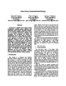
where the columns of U and V contain the spatial (topo) and temporal (chrono) singular vectors respectively, V ∗ denotes the conjugate transpose of V , and the diagonal elements of A are the Na = min(Nc , Ns′ ) non-negative sin′ gular values. The set of topos (chronos) are an orthonormal basis of RNc (Ns ) . The convention is for the singular values to be sorted in decreasing monotonic order meaning that A is independent of the ordering of the channels within S. Shown in figure 1 are singular values from a typical H1 Mirnov dataset. From the chronos power spectra we see that there are two dominant modes, each with two singular values suggesting they are both travelling waves, as discussed below. We also see that the variance-normalisation of each channel degrades the signal to noise ratio of the system, which can also be described in terms of the normalised entropy. We calculate the normalised entropy H of the singular values ak in A: H=

−

P Na

k=1 pk

log pk

log Na

,

(3)

where pk is the dimensionless energy: pk =

a2k , E

E=

Na X

a2k .

(4)

k=1

The low entropy case (H → 0) occurs when the system is well ordered. To some extent the scalar quantity H can be used as a measure of how physically interesting the signals in S are without any further investigation into the structure of S, though care must be taken with this interpretation. A standing wave in a system with no noise has only one non-zero singular value a0 = 1 giving H = 0, whereas a travelling wave requires two singular values so H > 0. 3

101

80

70

Singular Value

Frequency [kHz]

60

50

40

30

100

10-1

20

10

0

C0

C1

C2

C3

C4

10-2 0

C5

5

10

15

20

25

30

SV number

Fig. 1. Example of chronos power spectra and singular values. Singular values from both normalised (o) and unnormalised (x) S are shown. C0, C1, . . . , C5 denote the chronos from the normalised singular value 0, 1, . . . , 5. There are two distinct modes, one at f ∼ 45 kHz described by SV0 and SV1; the other, weaker, signal is at f ∼ 29 kHz and is described by SV2 and SV3. The data is from H1 shot #58122 at 31 < t < 32 ms.

2.3 Fluctuation structures Recognising that a travelling wave structure consists of a pair of singular values which naturally belong together we group similar singular values, defining a fluctuation structure α as a subset of singular values which have chronos with similar power spectra. We measure the similarity between two chronos c1 and c2 with the normalised average of the cross-power spectrum γc1,c2 : γc1 ,c2 =

G(c1 , c2 )2 , G(c1 , c1 )G(c2 , c2 )

(5)

where G(a, b) = h|F (a)F ∗(b)|i, F is the Fourier transform, and h. . .i represents the spectral average. When allocating singular values to fluctuation structures, the observation: γa,b > γmin

and γa,c > γmin

;

γb,c > γmin ,

(6)

suggests that we should not simply seek to require γa,b > γmin for each pair of singular values a, b within a structure, instead we follow the process in algorithm 1. In so doing we therefore require that each constituent singular vector has sufficient γ with the dominant singular vector of the structure. Various possible fluctuation structures for the dataset of figure 1 are shown in figure 2 as a function of the threshold value γmin . At γmin = 0, all singular 4

while Number of unallocated singular values > 0 do Define a new fluctuation structure as an empty set of singular values: αi = {} Denote the largest unallocated singular value by aξ for Every unallocated singular value aζ do if γζ,ξ > γmin then Allocate aζ to fluctuation structure αi end if end for end while Algorithm 1: Building fluctuation structures αi from singular values aj . The largest unallocated singular value aξ will always be allocated to αi because γξ,ξ = 1.

γmin=0.7

Fluctuation structure energy

1.0

0.8

{a0,a1}

0.6

{a2,a3,a5,a6}

0.4

{a2,a3}

a0 a1

0.2

a2 a3 0.0 0.0

0.2

0.4

γmin

0.6

0.8

1.0

Fig. 2. The possible fluctuation structure groupings according to their energies as defined by algorithm 1 through the range of γmin . The dataset is the same as in figure 1. We see that γmin . 0.4 allows unrelated singular values to be included within a fluctuation structure, whereas with γmin > 0.87 algorithm 1 will not recognise the similarity between a2 and a3 .

values are grouped together as a single fluctuation structure, while at γmin = 1 each fluctuation structure contains one singular value. The key features are the two fluctuation structures α0 = {a0 , a1 } and α1 = {a2 , a3 } which coexist for 0.50 < γmin < 0.87. After application of such analysis to a suitably sized sample of short time segments, a threshold of γmin = 0.7 was found to be appropriate for our dataset. 5

2.4 Data filtering

Filters are applied to the dataset in order to reduce its size and to remove noise. Two values which can be used to quantify the quality of the data are the normalised energy p and normalised entropy H. The normalised energy p of a fluctuation structure is defined as the sum of the normalised energies of its constituent singular values from equation 4. The nature of these thresholds is quite different; H thresholds will act upon the entire short time segments, whereas p thresholds affect individual fluctuation structures. Using a normalised energy threshold value p′ allows filtering out of low energy noise. As seen in our example dataset (figure 3), there appears to be a clear distinction between higher energy fluctuations (p & 0.6) and lower energy noise (p . 0.2). The use of H thresholds is not always appropriate, especially if spectra are present with several distinct fluctuations; in such cases if the dataset needs to be reduced in size it is preferable to simply use a random subset of the data. Entropy filtering is generally more useful when a significant number of S contain only noise. An alternative to using a hard p threshold uses an energy threshold defined as a fraction of the possible range of normalised energy for a given singular value, before constructing fluctuation structures. This method is more sensitive to modes which have reduced pk due to the coexistence of other modes. The nth largest singular value in a given short time segment has, by definition, a maximal normalised energy of 1/n. We then apply a factor p∗ , where 0 < p∗ < 1, and, starting with the smallest singular value, retain singular values with pn ≥ p∗ /n. Any point retained brings in all larger singular values from the same time segment, trumping the pn ≥ p∗ /n condition for lower n. The requirement for bringing in larger singular values is easily understood by considering the case of a mode having two singular values of almost equal energy, it is possible for the lower energy value to exceed the threshold with the higher value below the threshold.

2.5 Mapping of fluctuation structures into ∆ψ-space We regard each fluctuation structure as a point in the space [−π, π]Nc , an Nc – dimensional torus of length 2π which we will call ∆ψ-space. In this application ψ represents the electrical phase of the reconstructed fluctuation structure at the positions of the coils. Fluctuation structures which are close in ∆ψspace can be considered the same type. This interpretation arises from the expectation that the possible waves have various phase velocities and mode numbers due to the periodic boundary conditions of the physical plasma torus 6

1.0

0.8

p

0.6

0.4

0.2

0.0 0.2

0.4

0.6

H

0.8

1

10

2

3

10

10

Nα

4

10

0

20

40

60

pN α

80

100 120

Fig. 3. A 10% random sample of a dataset. The left panel shows p and H for the fluctuation structures. The middle panel shows the number of fluctuation structures Nα within δp = 0.01. The right panel shows pNα , which is effectively the density of normalised energy; while this is not physically meaningful because the normalisation factor is dependent on short time segment, it is a useful guide to the energy distribution among fluctuation structures.

in which they propagate. It is also applicable to the more general case where waves are spatially localised within the system and do not have well defined mode numbers. For each fluctuation structure αl we take the inverse SVD to get Sl : Sl = UAl V ∗ ,

(7)

where the elements of A not in αl are set to zero to form Al . The rows of the matrix Sl contain the timeseries relating to αl for each channel. In general, the power spectra of the topos in αl are peaked around a single frequency ωl . The phase differences ∆ψa,b (ω = ωl ) between channels a and b evaluated at ω = ωl are used to define the coordinates in ∆ψ-space. Using phase differences between each pair of channels would result in a 21 Nc (Nc −1)-dimensional space; instead we use the Nc −dimensional space of only nearest neighbour channels. Note that in our example dataset the actual phase difference between channels depends on κh so we map the phase differences to a coordinate system which is independent of κh , namely the κh -averaged magnetic angles of the Mirnov coils. 7

120

f [kHz]

100 80 60 40 20

0.15

0.00 0.0

0.2

0.4

κh

0.6

7/5

4/3

5/4

0.05

6/5

0.10

7/6

[m]

0 0.20

0.8

1.0

Fig. 4. The preprocessed dataset: In the upper panel, fluctuation structures are mapped to frequency and the magnetic geometry parameter κh , marker size and colour are proportion to the normalised energy of the fluctuation structure. In the lower panel, the average minor radial hri locations of low order rational magnetic surfaces are shown.

2.6 An overview of the preprocessed dataset As an overview of the preprocessed dataset, figure 4 shows the fluctuation structures with energy p > 0.2 mapped to the magnetic geometry parameter κh ; the radial location of low-order rational magnetic surfaces, ι = n/m, are also shown. These rational surfaces are important as fluctuations with toroidal and poloidal mode numbers n and m respectively can resonate with the twisted field lines. The main features of the fluctuation spectra are the resonances about κh = 0.4 and κh = 0.76, related to the ι = 5/4 and ι = 4/3 surfaces respectively. We expect that any automated process used to locate distinct types of fluctuations would identify these features, and hopefully find some less obvious features. Indeed in section 4 it can be seen that these two features are the first to be distinguished by the following clustering algorithm.

3

Clustering

We aim to discover any underlying lower-dimensional model of the dataset; that is, groups of fluctuation structures which are similar throughout some 8

range of short time segments. As discussed in section 2.5, we assume that a class of fluctuations is localised in the Nc -dimensional ∆ψ-space. For example, it is simple to understand such localisation in terms of a simple cylindrical geometry with equidistant poloidal measurements, where each mode with poloidal mode number m will be located at ∆ψ = 2πm/Nc in each dimension. However, we assume a generalised case in which the fluctuation may have arbitrary, including localised, structure. Many different types of clustering algorithms exist; here we use the expectation maximisation (EM) algorithm which is a method for estimating the most likely values of latent variables in a probabilistic model[5]. Here we assume that each type of fluctuation can be described by a Nc -dimensional Gaussian distribution in ∆ψ space. The latent variables are the mean µi and standard deviation σi for each cluster i, where i = 1, 2, 3, . . . , NCl and NCl is the number of clusters. Given the initial conditions, in the form of random initial µi and σi values for a prescribed number of clusters, the EM algorithm consists of two steps which repeat until a convergence criterion is met. Firstly, the expectation step assigns to each datapoint a probability, or expectation value, of belonging to each cluster which is calculated with the Gaussian distribution function. Secondly, µi and σi are recalculated using the new expectation values as weight factors. The 10-fold cross-validated log-likelihood ratio is used as a measure of how well the cluster assignments fit the data. The cross-validation process involves partitioning the dataset into random subsamples and comparing results from each subset to avoid oversensitivity to outliers in the data. The likelihood is the conditional probability of obtaining the cluster means and standard deviations given the observed data. Because the EM algorithm can only guarantee a local maximum in likelihood we use a Monte Carlo approach, with multiple repetitions with different randomised initial conditions for each NCl .

3.1 Visualisation

The identification of the correct number of clusters, or of those which are important, is a task that is by no means trivial to automate. We have found inspection of a dendrogram, or cluster tree, mapping to be a practical method for identifying the important clusters. The cluster tree displays clusters for each NCl below some maximum value NCl,max , with all clusters for a given NCl forming a single tree level. Each child cluster is mapped to the cluster on the parent level with which it has the largest fraction of common datapoints. Cluster branches which do not fork over a significant range of NCl are deemed to be well defined, and the point where well defined clusters start to break up suggests that NCl is too high. While this procedure is clearly a subjective one, 9

it is effective and does not depend on the type of clustering algorithm used. The cluster tree for our example dataset is shown in figures 5. Each cluster has been defined only by its phase structure ψ and mapped back to κh and frequency f = (2π)−1 ωl . The base of the tree (NCl = 1) shows all the data within a single cluster (EM:A); as we climb up the tree different classes of fluctuation are isolated. For example, the branch starting at cluster EM:B contains fluctuations with toroidal mode number n = 5 and poloidal mode number m = 4 which occur at configurations near the ι = 5/4 resonance (κh ≃ 0.4). Similarly, the branch containing cluster EM:C is due to the ι = 4/3 resonance near κh = 0.75. Other clusters include fluctuations which occur at higher order resonances, as well as low frequency n, m = 0 modes (cluster EM:O branch) and weakly defined residual clusters (EM:K and EM:L) which would be resolved at a higher level of the tree than is shown here. Shown in figure 6 are poloidal phase-angle plots for a single poloidal Mirnov array. The centre line corresponds to the cumulative mean phase of the coil pairs. The lines above and below are the cumulative cluster standard deviaPn−1 2 Pn−1 2 tions of the coil pairs, where σ1,n = j=1 σj,j+1 for ψ1,n = j=1 ∆ψj,j+1 . Here, the magnetic angles have been evaluated for a flux surface at r = 0.1 m to better represent the broad radial structure expected for these modes.

4

Discussion

The data mining algorithm presented here is potentially useful in numerous other domains where spatio-temporal data is used. However, there is a limitation to the nature of the fluctuations amenable to this analysis due to the SVD. The SVD is not effective in distinguishing different modes coexisting with the same frequency or spatial structure because the modes would share a chrono or topo, whereas the SVD requires orthogonal components to distinguish modes. The assumption that such coexisting modes are not present is also important in assigning a single frequency ωl to a fluctuation structure, i.e.: two modes with the same spatial structure will also share chronos, but only one frequency would be recorded. The EM clustering method described here relies on the assumption that clusters can be described by a Gaussian distribution. To check if the imposed Gaussian distributions significantly influence the cluster outcomes, we have also used the agglomerative hierarchical (AH) clustering algorithm [6] which does not make such an assumption. The initial condition for AH clustering is that each fluctuation structure defines a cluster. Using a suitable metric the two closest clusters are combined, iterating the process until we have NCl = 1 gives a (prohibitively large) cluster tree. Compression of the AH cluster tree 10

EM:O EM:E

EM:B

EM:M 10 (156)

2 (339)

EM:F

10 (168)

EM:G EM:A

3 (1309)

1 (2000)

EM:C

5 (433)

EM:D

EM:A

10 (308)

EM:I

10 (152)

1 (2000)

120 100 80 60 40 20 0

AH:A

(520)

EM:N

10 (57)

EM:L

10 (422)

EM:J

10 (95)

AH:B

(169)

AH:C

(164)

AH:D

EM:K

10 (352)

(104) AH:(Remainder) (884)

AH:E 0.0

EM:H

8 (96)

11 Freq. [kHz]

10 (128)

10 (162)

0.2

0.4

0.6

κh

0.8

(50)

AH:F

(40)

AH:G

(36)

AH:H

(33)

1.0

Fig. 5. Cluster tree of the example dataset. The figure in the bottom left corner is equivalent to figure 4; its upper panel shows the fluctuation structures mapped to f and κh , the numbers 1 (2000) at the top right are the tree level, NCl , and cluster population respectively, EM:A is a cluster label used for reference. For clarity, only a subset of clusters within the tree have their contents displayed and EM:G has been displaced to prevent overlap. Vertical parent-child distance is proportional to the distance between cluster means, while line thickness is inversely proportional to the Gaussian width of the cluster. Several clusters produced by the agglomerative hierarchical (AH: labels) method are also shown, these are essentially equivalent to the NCl = 10 level EM clusters, see table 1 for comparison.

4

2

3

1

4

2

Phase/2π

Phase/2π

Phase/2π

3 2

1

1

π

π/2

3π/2

0

-1

2π

π

π/2

3π/2

2π

-2

π

π/2

3π/2

Mean poloidal angle [r=0.1m]

Mean poloidal angle [r=0.1m]

Mean poloidal angle [r=0.1m]

(a) Cluster 47

(b) Cluster 48

(c) cluster 46

2π

Fig. 6. Variation of phase around one of the poloidal Mirnov arrays, plotted against mean magnetic poloidal coordinate. The centre line is the cumulative mean phase of the coil pairs, with standard deviation shown above and below. The mode numbers shown here are supported by Fourier analysis of the data. Cluster

AH:A

EM:H

307

EM:I

152

AH:B

AH:C

AH:D

AH:F

AH:G

AH:H

AH:(Rem.)

total

1

308 152

EM:E

161

EM:F

3

155 88

EM:O

50

EM:M EM:J

AH:E

3

28 40 36

EM:N EM:K

33

3

6

EM:L

25

2

3

16

5

1

162

10

168

40

128

78

156

52

95

21

57

289

352

392

422

total 520 169 164 104 50 40 36 33 884 Table 1 A comparison of populations of clusters produced by the EM (NCl = 10) and AH algorithms, clusters are shown in figure 5

can be achieved by filtering out clusters with small populations, allowing for a visualisation similar to the EM cluster tree in figure 5; a set of AH clusters which are essentially equivalent to the NCl = 10 level of the EM cluster tree are also shown in figure 5 . The clusters resulting from the EM and AH methods have been found to be essentially the same apart from the weakly defined clusters (EM:K,L) and the ‘remainder’ (AH:Rem), a quantitative comparison between populations of EM and AH clusters in figure 5 is shown in table 1. It is important to consider the scalability and computational requirements of the algorithm. Given fixed values of Nc and ∆t, the size of S remains 12

2000

constant and the preprocessing stage has complexity O(NS ), where NS is the number of timeseries datasets S. The scalability of the clustering stage depends on the algorithm used, for the EM case we have O(NCl Nα ), which gives O(NS ) for constant NCl . The AH clustering algorithm is less desirable as it has complexity O(Nα2 ) due to distance calculation between each pair of fluctuation structures. We have implemented the preprocessing and visualisation stages using the python language with the Scipy and Matplotlib libraries [7]. The preprocessing of our dataset, 4600 S arrays (28 by 1000), takes around 2 hours using a 1.9 GHz Intel Pentium M processor. The results are stored in MySQL tables; a table of fluctuation structure properties excluding ∆ψ-space mapping is around 5 Mb in size, with the 3.6 × 106 rows of the ∆ψ mapping table taking around 30 Mb, using optimal data types. For clustering, we have used the EM algorithm from the WEKA suite of data mining tools [8,9] which runs at about 0.05×NCl ×Nα CPU seconds using 2.2 GHz AMD Opteron processors. For each NCl , 100 randomised initial conditions were used; the results with maximal log-likelihood are selected as the best clusters. The WEKA algorithm does not operate with toroidal data, so we map the ∆ψ−space from the Nc -dimensional torus to a 2Nc -dimensional cube [−1, 1]2Nc by taking the sin(∆ψ) and cos(∆ψ) components. For the present work, no specific efforts were made to optimize the clustering process; more efficient clustering routines exist, including, for example, genetic algorithms for faster convergence. The physical nature of the fluctuations in our example dataset is not yet completely understood. The dependence of spectra on plasma density n and ι suggests a dispersion relation similar to that of the global Alfv´en eigenmode (GAE) [10,11]. However, the observed frequencies are smaller than the expected GAE frequencies by a factor of around 1/3 [12]; an experimental campaign is presently being undertaken in order to resolve this difference.

5

Conclusion

We have presented a highly automated data mining process for the characterisation of fluctuations in multichannel timeseries data. The manual interaction is restricted to two tasks: the selection of a cross-power threshold γmin and the choice of appropriate filter parameters. The former requires initial consideration of threshold effectiveness on a small subset of data, while the latter is an operation applied to the dataset as a whole. Given an appropriate choice of clustering algorithm, the data mining process scales well, with complexity O(NS ). We have used the procedure here with magnetic fluctuation data from configuration scans in the H-1 heliac, identify13

ing different modes in parameter space. The process should be easily adaptable to other types of multichannel oscillatory timeseries data.

Acknowledgements The authors would like to thank the H-1 team for continued support of experimental operations as well as J. Harris, F. Detering and M. Hegland for useful discussions. This work was performed on the H-1NF National Plasma Fusion Research Facility established by the Australian Government, and operated by the Australian National University, with support from the Australian Research Council Grant DP0344361 and DP0451960.

References [1] S. M. Hamberger, B. D. Blackwell, L. E. Sharp and D. B. Shenton, H-1 design and construction. Fusion Technol. 17 (1990) 123–130 [2] J. H. Harris et al, Fluctuations and stability of plasmas in the H-1NF heliac. Nucl. Fusion 44 (2004) 279–286 [3] B. D. Blackwell, Results from helical axis stellarators, Phys. Plasmas 8 (2001) 2238–2244 [4] T. Dudok de Wit, A.-L. Pecquet, J.-C. Vallet and R. Lima, The biorthogonal decomposition as a tool for investigating fluctuations in plasmas. Phys. Plasmas. 1 (1994) 3288–3300 [5] A. Dempster, N. Laird and D. Rubin, Maximum likelihood from incomplete data via the EM algorithm. J. Royal Stat. Soc. 39 (1977) 1–38 [6] W. H. E. Day and H. Edelsbrunner, Efficient Algorithms for Agglomerative Hierarchical Clustering Methods, J. Classification 1 (1984) 7–24 [7] http://python.org, http://scipy.org, http://matplotlib.sourceforge.net [8] I. H. Witten and E. Frank, Data Mining: Practical machine learning tools and techniques, 2nd Edition, Morgan Kaufmann (2005) [9] http://www.cs.waikato.ac.nz/ml/weka [10] K. L. Wong, A review of Alfv´en eigenmode observations in toroidal plasmas, Plasma Phys. Control. Fusion 41 (1999) R1–R56 [11] D. A. Spong, R. Sanchez and A. Weller, Shear Alfv´en continua in stellarators, Phys. Plasmas 10 (2003) 3217–3224 [12] D. G. Pretty, PhD Thesis, Australian National University (2007)

14