A Simple, Fast Support Vector Machine Algorithm for Data Mining

A Simple, Fast Support Vector Machine Algorithm for Data Mining Thanh-Nghi Do 1, François Poulet 2 1

College of Information Technology, Cantho University 1 Ly Tu Trong Street, Ninh Kieu District Cantho City, Vietnam [email protected] 2 ESIEA Pôle ECD 38, rue des Docteurs Calmette et Guérin Parc Universitaire de Laval-Changé 53000 Laval - France [email protected]

Abstract. Support Vector Machines (SVM) and kernel related methods have shown to build accurate models but the learning task usually needs a quadratic programming, so that the learning task for large datasets requires big memory capacity and a long time. A new incremental, parallel and distributed SVM algorithm using linear or non linear kernels proposed in this paper aims at classifying very large datasets on standard personal computers. We extend the recent finite Newton classifier for building an incremental, parallel and distributed SVM algorithm. The new algorithm is very fast and can handle very large datasets in linear or non linear classification tasks. An example of the effectiveness is given with the linear classification into two classes of two million datapoints in 20-dimensional input space in some seconds on ten personal computers (3 GHz Pentium IV, 512 MB RAM, Linux).

1 Introduction In recent years, real-world databases increase rapidly (double every 9 months [11]). So the need to extract knowledge from very large databases is increasing. Knowledge Discovery in Databases (KDD [10]) can be defined as the non-trivial process of identifying valid, novel, potentially useful, and ultimately understandable patterns in data. Data mining is the particular pattern recognition task in the KDD process. It uses different algorithms for classification, regression, clustering and association. We are interested in SVM learning algorithms proposed by Vapnik [25] because they have shown practical relevance for classification, regression and novelty detection. Successful applications of SVMs have been reported for various fields, for example in face identification, text categorization and bioinformatics [13]. The approach is systematic and properly motivated by statistical learning theory. SVMs are the most well known algorithms of a class using the idea of kernel substitution [5]. SVM and kernel-based methods have become increasingly popular data mining tools. In spite of the prominent properties of SVM, they are not favorable to deal with the challenge of

large datasets. SVM solutions are obtained from quadratic programs (QP), so that the computational cost of an SVM approach is at least square of the number of training datapoints and the memory requirement making SVM impractical. There is a need to scale up learning algorithms to handle massive datasets on personal computers (PCs). The effective heuristics to improve SVM learning task are to divide the original QP into series of small problems [2], [4], [20], [21] incremental learning [3], [12], [23] updating solutions in growing training set, parallel and distributed learning [22] on PC network or choosing interested datapoints subset (active set) for learning [8], [24]. We have created a new algorithm that is very fast for building incremental, parallel and distributed SVM classifiers. It is derived from the finite Newton method for classification proposed by Mangasarian [17]. The new SVM algorithm can linearly classify two million datapoints in 20-dimensional input space into two classes in some seconds on ten PCs (3 GHz Pentium IV, 512 MB RAM, Linux). We briefly summarize the content of the paper now. In section 2, we introduce the finite Newton method for classification problems. In section 3, we describe how to build the incremental learning algorithm with the finite Newton method. In section 4, we describe our parallel and distributed versions of the incremental algorithm. We present numerical test results in section 5 before the conclusion in section 6. Some notations are used in this paper. All vectors will be column vectors unless transposed to row vector by a T superscript. The inner dot product of two vectors, x, y is denoted by x.y. The 2-norm of the vector x will be denoted by ||x||. The matrix A[mxn] will be m datapoints in the n-dimensional real space Rn. The classes +1, -1 of m datapoints are denoted by the diagonal matrix D[mxm] of -1, +1. e will be the column vector of 1. w, b will be the coefficients and the scalar of the hyper-plane. z will be the slack variable and C is a positive constant. I denotes the identity matrix.

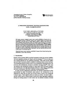
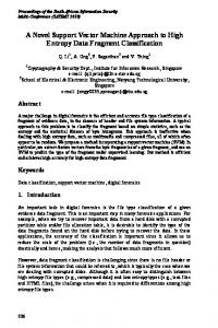
xT.w – b = -1

-1

xT.w – b = 0 xT.w – b = +1

+1

margin = 2/||w|| Fig. 1. Linear separation of the datapoints into two classes

2 Finite stepless Newton Support Vector Machine Let us consider a linear binary classification task, as depicted in figure 1, with m datapoints in the n-dimensional input space Rn, represented by the mxn matrix A, having corresponding labels ±1, denoted by the mxm diagonal matrix D of ±1. For this problem, the SVM algorithms try to find the best separating plane, i.e. furthest from both class +1 and class -1. It can simply maximize the distance or margin between the supporting planes for each class (xT.w – b = +1 for class +1, xT.w – b = -1 for class -1). The margin between these supporting planes is 2/||w|| (where ||w|| is the 2-norm of the vector w). Any point xi falling on the wrong side of its supporting plane is considered as an error (having corresponding slack value zi > 0). Therefore, a SVM algorithm has to simultaneously maximize the margin and minimize the error. The standard SVM formulation with a linear kernel is given by the following QP (1): Min f(w, b, z) = CeTz + (1/2)||w||2 s.t. D(Aw – eb) + z ≥ e (1) where slack variable z ≥ 0, constant C > 0 is used to tune errors and margin size. The plane (w, b) is obtained by the solution of the QP (1). Then, the classification function of a new datapoint x based on the plane is: predict(x) = sign(w.x – b) SVM can use some other classification functions, for example a polynomial function of degree d, a RBF (Radial Basis Function) or a sigmoid function. To change from a linear to non-linear classifier, one must only substitute a kernel evaluation in (1) instead of the original dot product. More details about SVM and others kernelbased learning methods can be found in [1] and [5]. Recent developments for massive linear SVM algorithms proposed by Mangasarian [17], [18] reformulate the classification as an unconstrained optimization. By changing the margin maximization to the minimization of (1/2)||w, b||2 and adding with a least squares 2-norm error, the SVM algorithm reformulation with linear kernel is given by the QP (2). Min f(w, b, z) = (C/2)||z||2 + (1/2)||w, b||2 s.t. D(Aw – eb) + z ≥ e (2) where slack variable z ≥ 0, constant C > 0 is used to tune errors and margin size. The formulation (2) can be rewritten by substituting for z = (e – D(Aw – eb))+ (where (x)+ replaces negative components of a vector x by zeros) into the objective function f. We get an unconstrained problem (3): Min f(w, b) = (C/2)||(e – D(Aw – eb))+||2 + (1/2)||w, b||2 By setting [w1 w2 … wn b]T to u and [A is rewritten by (4):

(3)

-e] to H, then the SVM formulation (3)

Min f(u) = (C/2)||(e – DHu)+||2 + (1/2)uTu

(4)

Algorithm 1. The finite stepless Newton SVM algorithm

- Input: training dataset represented by A and D matrices - Starting with u0 ∈ Rn and i = 0 - Repeat 1) ui+1 = ui - ∂2f(ui)-1∇f(ui) 2) i = i + 1 Until ∇f(ui) = 0 - Return ui Where the gradient of f at ui, ∇f(ui) = C(-DH)T(e – DHui)+ + ui

(5)

and the generalized Hessian of f at ui, ∂2f(ui) = C(-DH)Tdiag([e – DHui]*)(-DH) + I

(6)

with diag([e – DHui]*) denotes the (n+1)x(n+1) diagonal matrix whose jth diagonal entry is sub-gradient of the step function (e – DHui)+

Mangasarian [17] has shown that the finite stepless Newton method can be used to solve the strongly convex unconstrained minimization problem (4). The algorithm can be described as the algorithm 1. Mangasarian [17] has proved that the sequence {ui} of the algorithm 1 terminates at the global minimum solution. In most of the tested cases, the stepless Newton algorithm has given the good solution with a number of iterations varying between 5 and 8. The SVM formulation (4) requires thus only solutions of linear equations of (w, b) instead of QP. If the dimensional input space is small enough (less than 104), even if there are millions datapoints, the finite stepless Newton SVM algorithm is able to classify them in minutes on a PC. The algorithms can deal with non-linear classification tasks; however at the input of the algorithm 1, the training dataset represented by A[mxn] is replaced by the matrix the kernel matrix K[mxm], where K is a non linear kernel created by whole dataset A and the support vectors being A too, e.g.: - A degree d polynomial kernel of two datapoints xi, xj : K[i,j] = (xi.xj + 1)d - A radial basis kernel of two datapoints xi, xj : K[i,j] = exp(-γ|| xi – xj||2) The finite stepless Newton SVM algorithm using the kernel matrix K[mxm] requires very large memory size and execution time. Reduced support vector machine (RSVM) [15] creates rectangular mxs kernel matrix of size (s