It allows to debug wrong answers, that is, given an initial term we obtain either ... detect errors caused by wrong equations, membership axioms, and rewrite rules. ... In case of debugging a wrong rewrite computation, two different trees can be .... Reachable terms in one step When all the possible applications of each rule in ...
A Declarative Debugger for Maude Specifications User Guide∗ Adri´an Riesco, Alberto Verdejo, Rafael Caballero, and Narciso Mart´ı-Oliet Technical Report SIC-7-09 Departamento de Sistemas Inform´ aticos y Computaci´ on Universidad Complutense de Madrid
October 2009 (Revised November 12, 2010)
∗ Research supported by MEC Spanish projects DESAFIOS (TIN2006-15660-C02-01) and STAMP (TIN2008-06622C03-01), and Comunidad de Madrid program PROMESAS (S0505/TIC/0407).
Abstract We show in this guide how to use our declarative debugger for Maude specifications. Declarative debugging is a semi-automatic technique that starts from a computation considered incorrect by the user (error symptom) and locates a program fragment responsible for the error by asking questions to an external oracle, which is usually the user. In our case the debugging tree is obtained from a proof tree in a suitable semantic calculus; more concretely, we abbreviate the proof trees obtained from this calculus in order to ease and shorten the debugging process while preserving the correctness and completeness of the technique. We present the main features of our tool, what is assumed about the modules introduced by the user, the list of available commands, and the kinds of questions used during the debugging process. Then, we use several examples to illustrate how to use the debugger. We refer the interested reader to the webpage http://maude.sip.ucm.es/debugging, where these and other examples can be found together with more information about the theory underlying the debugger, its implementation and the Maude source files.
Contents 1 Preliminaries
3
2 Assumptions
4
3 Questions
5
4 Commands
6
5 Examples 5.1 Sorted lists . . . . . . . . . . . . . . . 5.2 WhileL semantics . . . . . . . . . . . . 5.2.1 WhileL evaluation semantics . 5.2.2 WhileL computation semantics 5.3 Heaps . . . . . . . . . . . . . . . . . . 5.4 Auction . . . . . . . . . . . . . . . . . 5.5 Solving a maze . . . . . . . . . . . . . 5.6 Vending machine . . . . . . . . . . . . 5.7 CCS semantics . . . . . . . . . . . . .
. . . . . . . . .
. . . . . . . . .
. . . . . . . . .
. . . . . . . . .
. . . . . . . . .
. . . . . . . . .
. . . . . . . . .
. . . . . . . . .
. . . . . . . . .
. . . . . . . . .
. . . . . . . . .
. . . . . . . . .
. . . . . . . . .
. . . . . . . . .
. . . . . . . . .
. . . . . . . . .
. . . . . . . . .
. . . . . . . . .
. . . . . . . . .
. . . . . . . . .
. . . . . . . . .
. . . . . . . . .
. . . . . . . . .
9 10 15 15 20 23 25 26 32 36
6 Graphical user interface 6.1 Debugging the sorted lists with the graphical interface . . . 6.2 Debugging a wrong rewrite: The WhileL semantics revisited 6.3 Debugging the heap with the GUI . . . . . . . . . . . . . . 6.4 Debugging the maze with the GUI . . . . . . . . . . . . . . 6.5 Debugging the vending machine with the GUI . . . . . . . .
. . . . .
. . . . .
. . . . .
. . . . .
. . . . .
. . . . .
. . . . .
. . . . .
. . . . .
. . . . .
. . . . .
. . . . .
. . . . .
. . . . .
. . . . .
. . . . .
. . . . .
. . . . .
. . . . .
. . . . .
. . . . .
. . . . .
44 44 48 53 54 55
. . . . . . . . .
. . . . . . . . .
. . . . . . . . .
. . . . . . . . .
. . . . . . . . .
. . . . . . . . .
. . . . . . . . .
. . . . . . . . .
. . . . . . . . .
. . . . . . . . .
. . . . . . . . .
1
Preliminaries
We present here the basic concepts and the main features of our declarative debugger, that will be referred through the rest of the paper. Declarative debugging, also known as algorithmic debugging, was first introduced by E. Y. Shapiro [7]. Declarative debugging is a semi-automatic technique that starts from a computation considered incorrect by the user (error symptom) and locates a program fragment responsible for the error. The declarative debugging scheme [4] uses a debugging tree as logical representation of the computation. Each node in the tree represents the result of a computation step, which must follow from the results of its child nodes by some logical inference. Diagnosis proceeds by traversing the debugging tree, asking questions to an external oracle (generally the user) until a so-called buggy node is found. A buggy node is a node containing an erroneous result, but whose children have all correct results. Hence, a buggy node has produced an erroneous output from correct inputs and corresponds to an erroneous fragment of code, which is pointed out as an error. From an explanatory point of view, declarative debugging can be described as consisting of two stages, namely the debugging tree generation and its navigation following some suitable strategy [8]. We present here a declarative debugger for Maude specifications. In our case the debugging tree is obtained from a proof tree in a suitable semantic calculus; more concretely, we abbreviate the proof trees obtained from this calculus in order to ease and shorten the debugging process while preserving the correctness and completeness of the technique; we refer to [5, 6] for more information about this topic. The current version of the tool has the following characteristics: • It allows to debug wrong answers, that is, given an initial term we obtain either a wrong term (due to a reduction or a rewrite) or a wrong membership computation. The debugger can be used to detect errors caused by wrong equations, membership axioms, and rewrite rules. • It also allows to debug missing answers. When working with functional modules, we consider not completely reduced normal forms and bigger than expected least sorts as missing answers. However, in a nondeterministic context such as Maude system modules, a missing answer is, given an initial term t, a bound in the number of steps n, and a condition c, a term reachable from t in at most n steps that fulfills c and that the system is not able to compute. In this kind of debugging, our tool is able to find errors due to wrong statements, missing rules, and errors in the condition imposed to the reachable terms. • It supports all kinds of modules: for example, operators can be declared with any combination of axiom attributes; equations can be defined with the otherwise attribute; modules can be parameterized; and operators’ arguments can be frozen (see [1] for the meaning of all these concepts). • The tool allows to debug specifications where some statements are suspicious and have been labeled (each one with a different label). Thus, the judgments related to the unlabeled statements will be considered correct and will not generate nodes in the debugging tree. The user is in charge of this labeling. • The user can decide to use all the labeled statements as suspicious or can use only a subset by trusting labels and modules. Moreover, the user can answer that he trusts the statement associated with the currently questioned judgment; that is, statements can be trusted “on the fly.” This produces that other nodes associated with the currently trusted statement are also deleted from the tree. • When debugging missing answers some operators and sorts can be pointed out as final, that is, the terms built with these operators at the top and constructed terms (i.e., terms built using only operators with the attribute ctor) having one of these sorts1 cannot be further rewritten. Final sorts can also be identified “on the fly,” removing the questions associated to the sort identified as final from the debugging tree. • Before starting the debugging process, the user can select a module containing only correct statements. By checking the correctness of the judgments with respect to this module the debugger can reduce the number of questions asked to the user. 1 Note
that if the least sort of a term is a subsort of one of these sorts, then the term will also be considered final.
3
• When debugging missing answers we consider that constructed terms are always in normal form, and thus the corresponding nodes will be deleted from the debugging tree. • It supports different kinds of searches when debugging missing answers: in zero or more steps, in one or more steps, and search of terms that cannot be further rewritten. • In case of debugging a wrong rewrite computation, two different trees can be built: one whose questions are related to one-step rewrites and another whose questions are related to several steps. The latter tree is partially built so that any node corresponding to a one-step rewrite is expanded only when the navigation process reaches it. • In the same way, when debugging missing answers the user can choose between two different trees: one whose questions are related to a set of terms obtained with just one rewrite step and another whose questions are associated with a set of terms obtained with several steps. • It provides two strategies to traverse the debugging tree: top-down, that traverses the tree from the root asking each time for the correctness of all the children of the current node, and then continues with one of the incorrect children; and divide and query, that each time selects the node whose subtree’s size is the closest one to half the size of the whole tree, keeping only this subtree if its root is incorrect, and deleting the whole subtree otherwise. • The condition imposed to the reachable terms when debugging missing answers can be defined in a very complicated way, but the user generally has in mind the terms that must fulfill it. Thus, the debugger allows to prioritize questions related to the fulfillment of the condition from questions involving the statements defining it. Moreover, if this option is used the trees proving whether the condition holds or not are built on demand, so they will be computed only if needed. • If the current question is too complicated the debugger allows to avoid it with a command don’t know. However, this command can introduce incompleteness. • The debugger provides an undo command, that allows the user to return to the previous state when an incorrect answer has been provided.
2
Assumptions
Since we are debugging Maude modules, they are expected to satisfy the appropriate executability requirements. The specifications in functional modules have to be terminating, confluent, sort decreasing and, given an equation t1 = t2 if C1 ∧ . . . ∧ Cn , all the variables occurring in t2 and C1 . . . Cn must appear in t1 or become instantiated by matching [1, Section 4.6]. While the equational part of system modules has to fulfill these requirements, rewrite rules must be coherent with respect to the equations and, given a rule t1 ⇒ t2 if C1 ∧ . . . ∧ Cn , the variables occurring in t2 and C1 . . . Cn must appear in t1 or become instantiated in matching or rewriting conditions [1, Section 6.3]. One interesting feature of our tool is that the user is allowed to trust some statements, by means of labels applied to the suspicious statements. This means that the unlabeled statements are assumed to be correct, and only their conditions will generate questions. In order to obtain a nonempty abbreviated proof tree, the user must have labeled some statements (all with different labels); otherwise, everything is assumed to be correct. In particular, the wrong statement must be labeled in order to be found. Likewise, when debugging missing answers some terms can be pointed out as final. Thus, this information has to be accurate in order to find the buggy node. Although the user can introduce a module importing other modules, the debugging process takes place in the flattened module. However, the debugger allows the user to trust a whole imported module. Navigation of the debugging tree takes place by asking questions to an external oracle, which in our case is either the user or another module introduced by the user. In both cases the answers are assumed to be correct. If either the module is not really correct or the user provides an incorrect answer, the result is unpredictable. Notice that the information provided by the correct module need not be complete, in the sense that some functions can be only partially defined. In the same way, it is not required to use the same signature in the correct and the debugged modules. If the correct module cannot help in answering a question, the user may have to answer it. Finally, the signature is supposed to be correct and will not be considered during the debugging process.
4
3
Questions
We briefly describe in this section the different kinds of questions asked by the debugger, defining for each of them when they are considered correct in order to answer appropriately them during the debugging process. The possible questions are related to: Reductions When a term t has been reduced by using equations to another term t0 , the debugger asks questions of the form “Is this reduction correct? t → t0 .” These judgments are correct if the user expected t to be fully reduced to t0 by using the equational part (equations and memberships) of the module. Normal forms When a term cannot be further reduced and it is not built only by constructors the debugger asks “Is t in normal form?,” which is correct if the user expected t to be a normal form. Memberships When a sort s is inferred for a term t, the debugger prompts questions of the form “Is this membership correct? t : s.” These judgments are correct if the expected least sort of t is a subsort of s or s itself. Least sorts When the judgment refers to the least sort ls of a term t, the tool makes questions of the form “Did you expect t to have least sort ls?” In this case, the judgment is correct if the intended least sort of t is exactly ls. Rewrites in one step When a term t is rewritten into another term t0 in only one step, the debugger asks questions of the form “Is this rewrite correct? t ⇒1 t0 ,” where t0 has already been fully reduced by using equations. This judgment is correct if the user expected to obtain t0 from t modulo equations with only one rewrite. Rewrites in several steps When a term t is rewritten into another one t0 after several rewrite steps, the debugger shows the question “Is this rewrite correct? t ⇒+ t0 ,” where t0 is fully reduced. This question is only prompted if the user selects the many-steps tree for wrong answers. This judgment is correct if t0 is expected to be reachable from t. Final terms When a term t cannot be further rewritten, the debugger asks “Did you expect t to be final?” This judgment is correct if the user expected that no rules can be applied to t. Solutions When a term t fulfills the search condition, the debugger shows questions of the form “Did you expect t to be a solution?” This judgment is correct if t is one of the intended solutions. In the same way, if a term does not fulfill the search condition the debugger asks “Did you expect t not to be a solution?,” that is correct if t is not one of the expected solutions. Reachable terms in one step When all the possible applications of each rule in the current specification to a term t lead to a set of terms {t1 , . . . , tn }, with n > 0, the debugger prompts the question “Are the following terms all the reachable terms from t in one step? t1 , . . . , tn .” This judgment is correct if all the expected terms from t in one step constitute the set {t1 , . . . , tn }. Reachable terms with one rule Given a term t and a rule r, when all the possible applications of r to t produces a set of terms {t1 , . . . , tn }, the debugger presents questions of the form “Are the following terms all the reachable terms from t with one application of the rule r? t1 , . . . , tn .” This judgment is correct if all the expected reachable terms from t with one application of r form the set {t1 , . . . , tn }. When n = 0 the debugger prompts questions of the form “Did you expect that no terms can be obtained from t by applying the rule r?,” that is correct if the rule r is not expected to be applied to t. Reachable terms in several steps Given an initial term t, a condition c, and a bound in the number of steps n, when all the terms reachable in at most n steps from t that fulfill c are t1 , . . . , tm , with m > 0, the debugger makes the following distinction: • If the condition c defines the initial condition of the search, the tool asks questions of the form “Are the following terms all the possible solutions from t in n steps? t1 , . . . , tm ,” where the bound is omitted if it is unbounded. This judgment is correct if all the solutions that the user expected to obtain from t in at most n steps constitute the set {t1 , . . . , tm }. If m = 0 the debugger asks questions of the form “Did you expect that no solutions are reachable from t in n steps?,” where the bound is again omitted if it is unbounded. In this case, the judgment is correct if no solutions were expected from t in at most n steps. 5
• If the condition c has been obtained from a rewrite condition t0 ⇒ p, then c is just a matching condition with the pattern p, and n is unbounded. In this case, the questions have the form “Are the following terms all the reachable terms from t that match the pattern p? t1 , . . . , tm .” This judgment is correct if all the terms that should be obtained from t and match the pattern p constitute the set {t1 , . . . , tm }. When m = 0 the questions have the form “Did you expect that no terms matching the pattern p can be obtained from t?,” that is correct if t is expected to be final or all the terms reachable from t are not expected to match p. These questions are only asked if the many-steps tree for missing answers is used. We recommend to follow some tips to ease the questions asked during the debugging process: • It is usually more complicated to answer questions related to many steps (both in wrong and missing answers) than questions related to one step. Thus, if a specification is complex it is better to debug it with a one-step tree. • There are some sorts that are usually final, such as Bool and Nat, so identifying them as final can avoid several tedious questions. • If an error is found using a complex initial term, this error can probably be reproduced with a simpler one. Using this simpler term leads to easier debugging sessions. • When facing a problem with both wrong and missing answers, it is usually better to debug first the wrong answers, because questions related to them are usually easier to answer and fixing them can also solve the missing answers problem. • When a question is related to a set of reachable terms that contains some wrong terms, it is recommended to point out one of these terms as erroneous instead of indicating the whole set as wrong. • When using the top-down navigation strategy, several questions are prompted. To point out one as erroneous or all of them as valid will shorten the debugging process, while pointing one question as correct usually only eases the current set of questions. Thus, to indicate that a question is valid is only recommended for extremely complicated or large sets of questions.
4
Commands
The debugger is initiated in Maude by loading the file dd.maude (available from http://maude.sip. ucm.es/debugging), which starts an input/output loop that allows the user to interact with the tool. Then, the user can enter Full Maude modules and commands, as well as commands for the debugger. The user can choose between using all the labeled statements in the debugging process (by default) or selecting some of them by means of the command (set debug select on .)
Once this mode is activated, the user can select and deselect statements by using2 (debug select LABELS .) (debug deselect LABELS .)
where LABELS is a list of statement labels separated by spaces. Moreover, all the labels in statements of a flattened module can be selected or deselected with the commands (debug include MODULES .) (debug exclude MODULES .)
where MODULES is a list of module names separated by spaces. It is also possible to specify which statements (equations, membership axioms or rules) are selected or deselected with the commands: 2 Although these labels, as well as the set of labels from a module and the final sorts below, can be selected and deselected with the corresponding modes switched off, they will have effect only when the corresponding modes are activated.
6
(debug include eqs/mbs/rls MODULES .) (debug exclude eqs/mbs/rls MODULES .)
where MODULES is a list of module names separated by spaces. The selection mode can be switched off by using the command (set debug select off .)
In a similar way, it is also possible to indicate that some terms are final, that is, that they cannot be further rewritten: • By using the value final in the attribute metadata of an operator, that indicates that the terms built with this operator at the top are final. • By selecting a set of final sorts. In this case, terms having one of these sorts (or having a subsort of these sorts) and built only with constructors (operators with the attribute ctor) are considered final. • On the fly, as will be explained below. In the first two cases, the user must activate the final sorts mode with the command (set final select on .)
While the attribute metadata must be written in the Maude file, final sorts can be selected/deselected with the commands (final select SORTS .) (final deselect SORTS .)
where SORTS is a list of sort identifiers separated by spaces. This option can be switched off with the command (set final select off .)
A module with only correct definitions can be used to reduce the number of questions. In this case, it must be indicated before starting the debugging process with the command (correct with MODULE-NAME .)
and can be deselected with the command (delete correct module .)
Since rewriting is not assumed to terminate, a bound, which is 42 by default, is used when searching in the correct module and can be set with the command (set bound BOUND .)
where BOUND is either a natural number or the constant unbounded. Note that if it is 0 the correct module will not be used, while if it is unbounded the correct module is assumed to be terminating. When debugging wrong rewrites, two different trees can be built: one whose questions are related to one-step rewrites and another whose questions are related to several steps. The user can switch between these trees, before starting the debugging process, with the commands (one-step tree .) (many-steps tree .)
being the first the default one. In the same way, when debugging missing answers we distinguish between trees whose nodes are related to sets of terms obtained with one (the default case) or many steps. The user can select them with the commands (one-step missing tree .) (many-steps missing tree .)
7
The generated debugging tree can be navigated by using two different strategies, namely, top-down and divide and query, being the latter the default one. The user can switch between them in any moment by using the commands (top-down strategy .) (divide-query strategy .)
When debugging missing answers, the user can prioritize questions related to the fulfillment of the search condition from questions involving the statements defining it. This option, switched off by default, can be activated with the command (solutions prioritized on .)
and can be switched off again with (solutions prioritized off .)
The debugging process for wrong answers is started with the commands (debug [in MODULE-NAME :] INITIAL-TERM -> WRONG-TERM .) (debug [in MODULE-NAME :] INITIAL-TERM : WRONG-SORT .) (debug [in MODULE-NAME :] INITIAL-TERM =>* WRONG-TERM .)
for wrong reductions, memberships, and rewrites, respectively. MODULE-NAME is the module where the computation took place; if no module name is given, the current module is used by default. Similarly, we start the debugging of missing answers with the commands (missing (missing (missing (missing (missing
[in MODULE-NAME :] INITIAL-TERM -> NORMAL-FORM .) [in MODULE-NAME :] INITIAL-TERM : LEAST-SORT .) [[depth]] [in MODULE-NAME :] INITIAL-TERM =>* PATTERN [s.t. CONDITION] .) [[depth]] [in MODULE-NAME :] INITIAL-TERM =>+ PATTERN [s.t. CONDITION] .) [[depth]] [in MODULE-NAME :] INITIAL-TERM =>! PATTERN [s.t. CONDITION] .)
where the first command debugs erroneous normal forms, the second one erroneous least sorts, and the remaining ones refer to incomplete sets found when using search. More specifically, the third specifies a search in zero or more steps, the fourth one in one or more steps, and the last one only checks final terms. The depth argument indicates the bound in the number of steps allowed in the search, and it is considered unbounded when omitted, while MODULE-NAME has the same behavior as in the commands above. How the process continues depends on the selected strategy. In the divide and query strategy, each question refers to one judgment that can be either correct or wrong. The different answers are transmitted to the debugger with the answers (yes .) (no .)
If the question asked is too difficult, the user can avoid to answer it with3 (don’t know .)
In addition to these general answers, others can be introduced depending on the kind of question. If it corresponds to the application of a statement, instead of just answering yes, we can also trust the statement on the fly if we decide the bug is not there. To trust the current statement we answer (trust .)
If a question refers to a set of reachable terms and one of these terms is not reachable, the user can point it out with the answer (I is wrong .) 3 Notice
that the question will not be asked again, thus this answer can lead to incompleteness.
8
where I is the index of the wrong term in the set. With this answer the debugger focuses on debugging this wrong judgment. In case the question is related to a set of reachable solutions, if one of the solutions is reachable but it should not fulfill the search condition, the user can indicate it with (I is not a solution .)
where I is the index of the term that should not be in the set. With this answer the user indicates that the definition of the search condition is erroneous and the debugger centers on it to continue the process. If the question is about a final term, additional information can be given by answering (its sort is final .)
that indicates to the debugger that all the constructed terms with the same sort as this term are final. In case the top-down strategy is selected, several questions will be displayed in each step. The user can introduce then answers of the form (N : answer .), where N is the index of the question and answer is the same answer that would be used in the divide and query strategy for this question. Thus, if there is an invalid question, the user can point it out with the answer (N : no .)
while correct questions are answered with (N : yes .)
As a shortcut to answer (yes .) to all the questions, the debugger provides the answer (all : yes .)
When the user considers that a question is too complicated, it can be discarded with (N : don’t know .)
If one of the questions is associated to a program statement and the user decides that it can be trusted, it is indicated with (N : trust .)
When a question presents a judgment from a term to a set of terms, and the term in position I is not reachable from the initial one, then we can point it out with (N : I is wrong .)
focusing the debugging process on this wrong computation. Furthermore, if the question refers to the set of reachable solutions, we can identify a reachable term that does not fulfill the search condition with the command (N : I is not a solution .)
where I the index of the term in the set. With this answer the debugger concentrates on the definition of the search condition. If one of the questions is related with a final term, on the fly information is given with (N : its sort is final .)
Finally, we can return to the previous state in both strategies by using the command (undo .)
5
Examples
We use in this section several examples to illustrate how to use the debugger. First, we debug wrong answers in functional and system modules by fixing the specifications of sorted lists and the operational semantics of a simple imperative language, WhileL [2]. Then, we describe how to debug missing answers by using a specification to find the exit in a labyrinth, the specification of a vending machine, and the description of the semantics of CCS [3]. 9
5.1
Sorted lists
We specify sorted lists by using a module parameterized by the theory TOSET [1, Section 8.3], that requires a sort Elt and a total order _ List{X} [ctor assoc] .
We define now when a list (with more than one element) is sorted by means of a membership axiom. It states that the first element must be smaller than the first of the rest of the list, and that the rest of the list must also be sorted: vars E E’ : X$Elt . var L : List{X} . var OL : SortedList{X} . cmb [olist] : E L : SortedList{X} if E X$Elt . eq [hd1] : head(E) = E . eq [hd2] : head(L E) = E .
We also define a sort function which sorts a list by successively inserting each element in the appropriate position in the sorted sublist formed by the elements previously considered: op insertion-sort : List{X} -> SortedList{X} . op insert-list : SortedList{X} X$Elt -> SortedList{X} . eq [is1] : insertion-sort(E) = E . eq [is2] : insertion-sort(E L) = insert-list(insertion-sort(L), E) . ceq [il1] : insert-list(E, E’) = E’ E if E’ < E . eq [il2] : insert-list(E, E’) = E E’ [owise] . ceq [il3] : insert-list(E OL, E’) = E E’ OL if E’ (red insertion-sort(3 4 7 6) .) result SortedList{NatAsToset}: 6 3 4 7
However, the list obtained is not sorted. Moreover, Maude infers that it is sorted. We can debug the buggy specification with the default divide and query strategy by using the command: Maude> (debug insertion-sort(3 4 7 6) -> 6 3 4 7 .)
With this command the debugger computes the tree shown in Figure 1, where the abbreviation is stands for insertion-sort, il for insertion-list, hd for head, and SL for SortedList{NatAsToset}. The first question asked by the debugger is: 10
is(6) → 6
is1
il(6, 7) → 6 7
is(7 6) → 6 7
hd(7) → 7
il2 is2
hd1 olist
6 7 : SL il(6 7, 4) → 6 4 7
is(4 7 6) → 6 4 7
il3
hd(4 7) → 7
hd2
4 7 : SL
6 4 7 : SL
is2
il(6 4 7, 3) → 6 3 4 7
is(3 4 7 6) → 6 3 4 7
hd1
hd(7) → 7
olist olist
il3 is2
Figure 1: Debugging tree for the sorted lists example
is(6) → 6
is1
il(6, 7) → 6 7
is(7 6) → 6 7
hd(7) → 7
il2 is2
hd1 olist
6 7 : SL il(6 7, 4) → 6 4 7
is(4 7 6) → 6 4 7
il3 is2
Figure 2: Debugging tree after the first answer Is this reduction (associated with the equation is2) correct? insertion-sort(4 7 6) -> 6 4 7 Maude> (no .)
We expect insertion-sort to order the list, so we answer negatively and the subtree shown in Figure 2 is selected to continue the debugging. The next question is: Is this reduction (associated with the equation il3) correct? insert-list(6 7,4) -> 6 4 7 Maude> (no .)
Since we expected 4 to be inserted in the first position we answer no, and the subtree corresponding to this reduction is selected as debugging tree (Figure 3). The debugger asks now the question: Is this membership (associated with the membership olist) correct? 6 7
: SortedList{NatAsToset}
Maude> (yes .)
This membership assertion is correct, so the subtree corresponding to this membership is deleted (Figure 4). With this information the debugging tree has been reduced to a leaf, and the debugger can conclude that it is associated with the wrong equation: The buggy node is: insert-list(6 7, 4) -> 6 4 7 with the associated equation: il3
That is, the debugger points to the equation il3 as buggy. If we examine it: ceq [il3] : insert-list(E OL, E’) = E E’ OL if E’ (red 6 3 4 7 .) result SortedList{NatAsToset}: 6 3 4 7
we can see that Maude continues assigning to it an incorrect sort. We debug this computation by using the command: Maude> (debug 6 3 4 7 : SortedList{NatAsToset} .)
The first question the debugger asks is: Is this membership (associated with the membership olist) correct? 3 4 7
: SortedList{NatAsToset}
Maude> (yes .)
Of course, this list is sorted. The following question is: Is this reduction (associated with the equation hd2) correct? head(3 4 7) -> 7 Maude> (no .)
But the head of a list should be the first element (on the left), not the last one, so we answer no. With only these two questions the debugger prints: The buggy node is: head(2 5 7) -> 7 with the associated equation: hd2
If we check the equation hd2, we can see that we take the element from the wrong side. The right equation is: eq [hd2] : head(E L) = E .
To debug this module we have used the default divide and query strategy. We illustrate now how to do it with the top-down strategy. We debug again the judgment insertion-sort(3 4 7 6) -> 6 3 4 7 in the initial module with the two errors: Maude> (top-down strategy .) Top-down strategy selected. Maude> (debug insertion-sort(3 4 7 6) -> 6 3 4 7 .)
The debugger asks now about the validity of the children of the root of the tree in Figure 1:
12
Question 1 : Is this reduction (associated with the equation is2) correct? insertion-sort(4 7 6) -> 6 4 7 Question 2 : Is this reduction (associated with the equation il3) correct? insert-list(6 4 7,3) -> 6 3 4 7 Maude> (1 : no .)
Both questions are wrong, so we select, for example, the first one. The debugger selects the associated node as the current one and asks about the validity of its children: Question 1 : Is this reduction (associated with the equation is2) correct? insertion-sort(7 6) -> 6 7 Question 2 : Is this reduction (associated with the equation il3) correct? insert-list(6 7,4) -> 6 4 7 Maude> (2 : no .)
This time, only one of the questions is wrong, so we select it. The debugger prints now: Question 1 : Is this membership (associated with the membership olist) correct? 6 7 : SortedList{NatAsToset} Maude> (1 : yes .)
There is only a question, and it is correct, so we give this information to the debugger, and it detects the wrong equation: The buggy node is: insert-list(6 7,4) -> 6 4 7 with the associated equation: il3
But remember that we chose a question randomly when the debugger showed two wrong questions. What happens if we select the other one? The following question is printed: Question 1 : Is this membership (associated with the membership olist) correct? 6 4 7 : SortedList{NatAsToset} Maude> (1 : no .)
Since this single question is wrong, we choose it and the debugger asks: Question 1 : Is this reduction (associated with the equation hd2) correct? head(4 7) -> 7 Question 2 : Is this membership (associated with the membership olist) correct? 4 7 : SortedList{NatAsToset} Maude> (1 : no .)
13
The first question is the only one erroneous, so we select it. With this information, the debugger prints: The buggy node is: head(4 7) -> 7 with the associated equation: hd2
That is, the second path finds the other bug. In general, this strategy may find different bugs if the user selects different wrong questions. In order to prune the debugging tree, we consider a module defining the sorting function sort in a correct, although inefficient, way. This module will define the functions insertion-sort and insert-list by means of sort: (fmod CORRECT-SORTING{X :: TOSET} is sorts List{X} SortedList{X} . subsorts X$Elt < SortedList{X} < List{X} . vars E E’ : X$Elt . vars L L’ : List{X} . var OL : SortedList{X} . op __ : List{X} List{X} -> List{X} [ctor assoc] . cmb if cmb if
E E E E
E’ : < E’ E’ L < E’
SortedList{X} . : SortedList{X} /\ E’ L : SortedList{X} .
op sort : List{X} -> SortedList{X} . ceq sort(L E E’ L’) = sort(L E’ E L’) if E’ < E . ceq sort(L E E’) = sort(L E’ E) if E’ < E . ceq sort(E E’ L) = sort(E’ E L) if E’ < E . ceq sort(E E’) = E’ E if E’ < E . eq sort(L) = L [owise] . op insertion-sort : List{X} -> SortedList{X} . op insert-list : SortedList{X} X$Elt -> SortedList{X} . eq insertion-sort(L) = sort(L) . eq insert-list(OL, E) = sort(E OL) . endfm)
We can use this module (instantiated with the view NatAsToset) to prune the debugging trees built by the debug commands if we previously introduce the command: Maude> (correct module CORRECT-SORTING{NatAsToset} .) CORRECT-SORTING{NatAsToset} selected as correct module.
Now we try to debug the initial module (with two errors) again. In this example, all the questions about correct judgments have been pruned, so all the answers are negative. In general, the correct module need not be complete, so some correct judgments could be presented to the user: Maude> (debug in SORTED-LIST-TEST : insertion-sort(3 4 7 6) -> 6 3 4 7 .) Is this transition (associated with the equation il3) correct? insert-list(6 4 7,3) -> 6 3 4 7 Maude> (no .) Is this membership (associated with the membership olist) correct?
14
6 4 7
: SortedList{NatAsToset}
Maude> (no .) Is this transition (associated with the equation hd2) correct? head(4 7) -> 7 Maude> (no .) The buggy node is: head(4 7) -> 7 with the associated equation: hd2
The correct module also improves the debugging of the membership. With only one question we discover the buggy equation: Maude> (debug in SORTED-LIST-TEST : 6 3 4 7 : SortedList{NatAsToset} .) Is this transition (associated with the equation hd2) correct? head(3 4 7) -> 7 Maude> (no .) The buggy node is: head(3 4 7) -> 7 with the associated equation: hd2
5.2
WhileL semantics
We illustrate how to debug wrong answers in system modules with the semantics of WhileL, a very simple programming language with arithmetic and Boolean expressions, assignments, sequential composition, conditionals, and loops [2, 10]. 5.2.1
WhileL evaluation semantics
This section describes the specification of the evaluation semantics of WhileL. First, we define the syntax of the language. We define sorts for the arithmetic and Boolean variables, operators, expressions, commands, and programs: (fmod WHILEL-SYNTAX is pr QID . sorts Var BVar Num Boolean Op BOp Exp BExp Com Prog . subsorts Qid < Var < Exp . subsort Nat < Num < Exp . ops w x y z : -> Var . ops +. -. *. : -> Op . op ___ : Exp Op Exp -> Exp [prec 20] . subsorts Qid < BVar < BExp . subsort Boolean < BExp . ops T F : -> Boolean . ops And Or : -> BOp . op ___ : BExp BOp BExp -> BExp [prec 20] . op Not_ : BExp -> BExp [prec 15] . op Equal : Exp Exp -> BExp .
15
We define the following commands: skip, assignment, concatenation of commands, conditional, and while loop. The fact that a command is a specific case of program is reflected in our signature by a subsort declaration: op op op op op
skip : -> Com . _:=_ : Var Exp -> Com [prec 30] . _;_ : Com Com -> Com [assoc prec 40] . If_Then_Else_ : BExp Com Com -> Com [prec 50] . While_Do_ : BExp Com -> Com [prec 60] .
subsort Com < Prog . endfm)
The evaluation of arithmetic and Boolean expressions is defined for each operator by using the Maude predefined functions: (fmod AP is pr WHILEL-SYNTAX . op Ap : Op Num Num -> Num . vars n n’ : Num . eq [plus] : Ap(+., n, n’) = n + n’ . eq [times] : Ap(*., n, n’) = n * n’ . eq [sd] : Ap(-., n, n’) = if n < n’ then 0 else sd(n, n’) fi . op Ap : BOp Boolean Boolean -> Boolean . var bv bv’ : Boolean . eq [andT] : Ap(And, T, bv) eq [andF] : Ap(And, F, bv) eq [orT] : Ap(Or, T, bv) = eq [orF] : Ap(Or, F, bv) = endfm)
= bv . = F . T . bv .
The environment, defined in the module ENV below, keeps the value associated to each variable: (fmod ENV is inc WHILEL-SYNTAX . sorts Value Variable ENV . subsorts Num Boolean < Value . subsorts Var BVar < Variable . op mt : -> ENV . op _=_ : Variable Value -> ENV [prec 20] . op __ : ENV ENV -> ENV [assoc id: mt prec 30] .
The module also defines look up and update functions. In case a variable has been assigned more than one value, the leftmost assignment is the newest and all the others can be deleted: op _[_] : ENV Var -> Num . op _[_] : ENV BVar -> Boolean . op _[_/_] : ENV Value Variable -> ENV [prec 35] . vars X X’ : Variable . vars V W : Value . var rho : ENV . var n : Num . var x : Var . eq [env1] : rho [V / X] = (X = V) rho .
16
eq [env2] : (X = V rho)[X’] = if X == X’ then V else rho[X’] fi . eq [env3] : (X = V) rho (X = W) = (X = V) rho . endfm)
The evaluation semantics of the language is described in the module EVALUATION. We use pairs of expressions or commands with environments (called statements) to obtain the result of the execution of a program: (fmod EVALUATION-EXP is pr ENV . pr AP . sort Statement . subsorts Num Boolean ENV < Statement . op : Exp ENV -> Statement . op : BExp ENV -> Statement . var var vars var vars var var var vars
x : Var . st : ENV . e e’ : Exp . op : Op . v v’ : Num . bx : BVar . bv bv’ : Boolean . bop : BOp . be be’ : BExp .
rl [CR] : < n, st > => n . rl [VarR] : < X, st > =>
st(X) .
crl [OpR] : < e op e’, st > => Ap(op,v,v’) if < e, st > => v /\ < e’, st > => v’ . rl [BCR1] : < T, st > => T . rl [BCR2] : < F, st > => F . rl [BVarR] : < bx, st > =>
st(bx) .
crl [BOpR] : < be bop be’, st > => Ap(bop,bv,bv’) if < be, st > => bv /\ < be’, st > => bv’ . crl [EqR1] : < Equal(e,e’), st > => T if < e, st > => v /\ < e’, st > => v . crl [EqR2] : < Equal(e,e’), st > => F if < e, st > => v /\ < e’, st > => v’ /\ v =/= v’ . crl [Not1] : if crl [Not2] : if endm)
< < <
=> F st > => T . be, st > => T st > => F .
We use this module to describe the semantics of statements: (mod EVALUATION-WHILE is protecting EVALUATION-EXP . subsort ENV < Statement .
17
op : Com ENV -> Statement . var X : Var . vars st st’ st’’ : ENV . var e : Exp . var v : Num . var be : BExp . vars C C’ : Com .
The assignment updates the environment with a new value for the variable: crl [AsR] : < X := e, st > => < skip, st[v / X] > if < e, st > => v .
The concatenation of statements evaluates the first command, and uses the result to evaluate the rest: crl [ComR] : < C ; C’, st > => < skip, st’’ > if < C, st > => < skip, st’ > /\ < C’, st’ > => < skip, st’’ > .
The conditional statement evaluates the condition and then selects the branch that must be evaluated: crl [IfR1] : < If be Then C Else C’, st > => < skip, st’ > if < be, st > => T /\ < C, st > => < skip, st’ > . crl [IfR2] : < If be Then C Else C’, st > => < skip, st’ > if < be, st > => F /\ < C’, st > => < skip, st’ > .
The while statement also distinguishes whether the condition is false or not. In the first case, it returns the same environment, while in the second one it evaluates the body of the loop: crl [WhileR1] : if crl [WhileR2] : if
< < < <
=> < skip, st > be, st > => F . While be Do C, st > => < skip, st’ > be, st > => T /\ C, st > => < skip, st’ > .
endm)
If we execute now the WhileL program below to multiply x = 2 and y = 3 and keep the result in z: Maude> (rew < z := 0 ; (While Not Equal(x, 0) Do z := z +. y ; x := x -. 1), x = 2 y = 3 z = 1 > .) result Statement : < skip, y = 3 z = 3 x = 1 >
we obtain z = 3, while we expected to obtain z = 6. Before starting the debugging process we can select a subset of the labeled statements as suspicious in order to avoid questions related to simple statements. To do it, we have to activate the selection mode: Maude> (set debug select on .) Debug select is on.
Now we have to select the set of labels that will be used during the debugging session. If we introduce a module as suspicious, all the labels in the flattened module will be suspicious. For example, if we state that the module EVALUATION-WHILE is suspicious, the labeled statements of all the modules in the specification are considered suspicious: Maude> (debug include EVALUATION-WHILE .) Labels andF andT env1 env2 env3 minus orF orT plus times AsR BCR1 BCR2 BOpR BVarR CR ComR EqR1 EqR2 IfR1 IfR2 Not1 Not2 OpR VarR WhileR1 WhileR2 are now suspicious.
18
If we check the specification, the arithmetic and Boolean operations defined in AP are simple enough to be trusted, so we can point it out with the command: Maude> (debug exclude AP .) Labels andF andT minus orF orT plus times are now trusted.
Moreover, the equations specifying the environment can also be trusted. Instead of introducing the whole module, we can introduce the trusted labels with the command: Maude> (debug deselect env1 env2 env3 .) Labels env1 env2 env3 are now trusted.
We can debug now the buggy behavior with the top-down strategy and the default one-step tree by typing the commands: Maude> (top-down strategy .) Top-down strategy selected. Maude> (debug < z := 0 ; (While Not Equal(x, 0) Do z := z +. y ; x := x -. 1), x = 2 y = 3 z = 1 > =>* < skip, y = 3 z = 3 x = 1 > .)
The debugger computes the tree and asks about the validity of the root’s children: Question 1 : Is this rewrite (associated with the rule AsR) correct? < z := 0,x = 2 y = 3 z = 1 > =>1 < skip,x = 2 y = 3 z = 0 > Question 2 : Is this rewrite (associated with the rule WhileR2) correct? < While z := x := x = 2
Not Equal(x,0)Do z +. y ; x -. 1, y = 3 z = 0 > =>1 < skip, y = 3 z = 3 x = 1 >
Maude> (2 : no .)
The second question is erroneous, because x has not reached 0, so we select this question, and the following questions are related to its children: Question 1 : Is this rewrite (associated with the rule Not2) correct? < Not Equal(x,0),x = 2 y = 3 z = 0 > =>1 T Question 2 : Is this rewrite (associated with the rule ComR) correct? < z := z +. y ; x := x -. 1, x = 2 y = 3 z = 0 > =>1 < skip, y = 3 z = 3 x = 1 > Maude> (all : yes .)
Since both questions are right, the debugger determines that the current node is buggy: The buggy node is: < While Not Equal(x,0) Do z := z +. y ; x := x -. 1, x = 2 y = 3 z = 0 > =>1 < skip, y = 3 z = 3 x = 1 > with the associated rule: WhileR2
19
If we examine now the WhileR2 rule we realize that the body of the while loop is evaluated only once. We fix this rule as follows: crl [WhileR2] : < While be Do C, st > => < skip, st’ > if < be, st > => T /\ < C ; (While be Do C), st > => < skip, st’ > .
If we execute now the program in the fixed module, we obtain the right result: Maude> (rew < z := 0 ; (While Not Equal(x, 0) Do z := z +. y ; x := x -. 1), x = 2 y = 3 z = 1 > .) result Statement : < skip, y = 3 z = 6 x = 0 >
5.2.2
WhileL computation semantics
In contrast to the evaluation semantics, the computation semantics describes the behavior of programs in terms of small steps [2, 10]. We define this behavior in the following module: (mod COMPUTATION-WHILE is protecting EVALUATION-EXP . op : Com ENV -> Statement . sort Statement2 . op (_,_) : Com ENV -> Statement2 . op Tick : -> Statement2 . var X : Var . vars st st’ : ENV . var e : Exp . var v : Num . var be : BExp . vars C C’ C’’ : Com . eq skip ; C = C . eq C ; skip = C . crl [AsRc] : < X := e, st > => < skip, st[v / X] > if < e, st > => v . crl [IfRc1] : < If be Then C Else C’, st > => < C’’, st’ > if < be, st > => T /\ < C, st > => < C’’, st’ > /\ C =/= C’’ . crl [IfRc2] : < If be Then C Else C’, st > => < C’’, st’ > if < be, st > => F /\ < C’, st > => < C’’, st’ > /\ C’ =/= C’’ . crl [ComRc1] : if crl [ComRc2] : if
< < < (
=> < C’’ ; C’, st > C, st > => < C’’, st’ > /\ C =/= C’’ . C ; C’, st > => < C’’, st’ > C, st ) => Tick /\ C’, st > => < C’’, st’ > /\ C’ =/= C’’ . < < <
While be be, st >
Do => Do =>
C, st > => < skip, st > F . C, st > => < C ; (While be Do C), st > T .
We also define the termination predicates for the language: rl [Skipt] : ( skip, st ) => Tick . crl [IfRt1] : ( If be Then C Else C’, st ) => Tick if < be, st > => T /\
20
H < A2 ; A3 , x = 5 y = 2 > ⇒f < A3 , x = 5 y = 2 > H < A1 ; A2 ; A3 , x = 5 y = 2 > ⇒f < A2 ; A3 , x = 5 y = 2 >
H < A3 , x = 5 y = 2 > ⇒f < skip, y = 2 x = 0 >
Tr
< A2 ; A3 , x = 5 y = 2 > ⇒+ < skip, y = 2 x = 0 >
< A1 ; A2 ; A3 , x = 5 y = 2 > ⇒+ < skip, y = 2 x = 0 >
Tr
Figure 5: Debugging tree for the computation semantics example
A � A � A � A � A� A � ComRc1 < A2 ; A3 , x = 5y = 2 > ⇒1 < A3 , x = 5y = 2 > < A3 , x = 5y = 2 > ⇒1 < skip,y = 2 x = 0 > < A2 ; A3 , x = 5y = 2 > ⇒+ < skip, y = 2x = 0 >
AsRc Tr
Figure 6: Debugging tree for the computation semantics example after the first answer ( C, st ) => Tick . crl [IfRt2] : ( If be Then C Else C’, st ) => Tick if < be, st > => F /\ ( C’, st ) => Tick . crl [ComRt] : ( C ; C’, st ) => Tick if ( C, st ) => Tick /\ ( C’, st ) => Tick . endm)
If we rewrite now a program to swap the values of two variables, their values are not exchanged: Maude> (rew < x := y := x := result Statement :
x x y
.) skip,y = 2 x = 0 >
We use the many-steps tree and the default divide and query strategy to debug this behavior: Maude> (many-steps tree .) Many-steps tree selected. Maude> (debug < x := x -. y ; y := x +. y ; x := y -. x, x = 5 y = 2 > =>* < skip, y = 2 x = 0 > .)
The tool builds the debugging tree shown in Figure 5 where the assignments in the program have been abbreviated as follows: A1 = x := x -. y, A2 = y := x +. y, A3 = x := y -. x. The debugging trees above ⇒f transitions have not been calculated yet (i.e., their premises have not been computed, represented by H); they are frozen until the navigation through the tree leads to them. A node is selected and the following question is presented to the user: Is this rewrite correct? < y := x +. y ; x := y -. x, x = 5 y = 2 > =>+ < skip, y = 2 x = 0 > Maude> (no .)
Notice the form =>+ of the arrow in the rewrite appearing in the question, to emphasize that it is a many-steps rewrite. The transition is wrong because the variables have not been properly updated. The debugger continues with the “defrost” tree shown in Figure 6, where the big triangles abbreviate the subtrees corresponding to the premises of each node, and asks the following question: Is this rewrite (associated with the rule ComRc1) correct? < y := x +. y ; x := y -. x, x = 5 y = 2 > =>1 < x := y -. x, x = 5 y = 2 > Maude> (no .)
21
st2
y = 2(y) → 2 st2 rmv2 x = 5 y = 2(x) → 5 x = 5 y = 2(y) → 2 remove(y = 2,y) → mt rmv2 VarR VarR ap-add < x,x = 5 y = 2 > ⇒1 5 < y,x = 5 y = 2 > ⇒1 2 Ap(+.,5,2) → 7 remove(x = 5 y = 2,y) → x = 5 st1 OpR < x +. y,x = 5 y = 2 > ⇒1 7 x = 5 y = 2[7 / y] → x = 5 y = 7 AsRc < y := x +. y,x = 5 y = 2 > ⇒1 < skip,x = 5 y = 7 > ComRc1 < y := x +. y ; x := y -. x,x = 5 y = 2 > ⇒1 < x := y -. x,x = 5 y = 2 > st2
Figure 7: Debugging tree for the computation semantics example after the second answer rmv2
remove(y = 2,y) → mt rmv2 remove(x = 5 y = 2,y) → x = 5 st1 x = 5 y = 2[7 / y] → x = 5 y = 7 AsRc < y := x +. y,x = 5 y = 2 > ⇒1 < skip,x = 5 y = 7 > < y := x +. y ; x := y -. x,x = 5 y = 2 > ⇒1 < x := y -. x,x = 5 y = 2 >
ComRc1
Figure 8: Debugging tree for the computation semantics example after the third answer This judgment is wrong because the values of the variables are not updated. Now the debugger selects the tree rooted by this node as current one (shown in Figure 7). The next question is: Is this rewrite (associated with the rule OpR) correct? < x +. y, x = 5 y = 2 > =>1 7 Maude> (trust .)
We consider that the application of a primitive operation is simple enough to be trusted. The remaining tree is shown in Figure 8. The next question is related to the application of an equation to update the store: Is this reduction (associated with the equation st1) correct? x = 5 y = 2[7 / y] -> x = 5 y = 7 Maude> (yes .)
This answers leads to the tree shown in Figure 9. Finally, a question about assignment is done: Is this rewrite (associated with the rule AsRc) correct? < y := x +. y, x = 5 y = 2 > =>1 < skip, x = 5 y = 7 > Maude> (yes .)
With this information, the debugger is able to find the bug: The buggy node is: < y := x +. y ; x := y -. x, x = 5 y = 2 > =>1 < x := y -. x, x = 5 y = 2 > with the associated rule: ComRc1
If we check the rule ComRc1 we realize that the store is not properly updated. The righthand side of the rule should be < C’’ ; C’, st’ >: crl [ComRc1] : < C ; C’, st > => < C’’ ; C’, st’ > if < C, st > => < C’’, st’ > /\ C =/= C’’ .
AsRc
< y := x +. y,x = 5 y = 2 > ⇒1 < skip,x = 5 y = 7 > < y := x +. y ; x := y -. x,x = 5 y = 2 > ⇒1 < x := y -. x,x = 5 y = 2 >
ComRc1
Figure 9: Debugging tree for the computation semantics example after the fourth answer 22
H H ComRc1 < A1 ; A2 ; A3 , x = 5 y = 2 > ⇒1 < A2 ; A3 , x = 5 y = 2 > < A2 ; A3 , x = 5 y = 2 > ⇒1 < A3 , x = 5 y = 2 > < A1 ; A2 ; A3 , x = 5 y = 2 > ⇒+ < A3 , x = 5 y = 2 >
ComRc1 Tr
Figure 10: Debugging tree for the computation semantics example using a correct module However, since we have the evaluation semantics of the language already specified and debugged, we can use that module as a correct module to reduce the number of questions to only one: Maude> (correct module EVALUATION-WHILE .) EVALUATION-WHILE
selected as correct module.
Maude> (debug in COMPUTATION-WHILE : < x := x -. y ; y := x +. y ; x := y -. x, x = 5 y = 2 > =>* < skip, y = 2 x = 0 > .)
After introducing these commands, the debugger builds the tree shown in Figure 10 and presents the following question: Is this rewrite (associated with the rule ComRc1) correct? < y := x +. y ; x := y -. x, x = 5 y = 2 > =>1 < x := y -. x, x = 5 y = 2 > Maude> (no .)
Having received a negative answer, the debugger tries to build the debugging tree associated to the left child in Figure 10 which had remained frozen until now. Such a tree is depicted in Figure 7; however, this time the information obtained from the correct module makes it possible to prune it so that the result consists only of the root. Having obtained a single node, it is pointed out as the buggy node: The buggy node is: < y := x +. y ; x := y -. x, x = 5 y = 2 > => < x := y -. x, x = 5 y = 2 > with the associated rule: ComRc1
5.3
Heaps
We show in this section how to specify in Maude binary heaps, that is, binary trees fulfilling that (1) all levels of the tree, except possibly the last one, are complete and, if the last level of the tree is not complete, the nodes of that level are filled from left to right; and (2) the contents of each node is greater than each of its children. The module HEAP defines binary trees (BTree) and Heaps and its nonempty variants (NeBTree and NeHeap), using a theory TH that defines the functions min, max, and a total order _ Heap [ctor] . op ___ : BTree X$Elt BTree -> NeBTree [ctor] .
We state by means of memberships when a binary tree is a heap: vars E E’ : X$Elt . vars L L’ R R’ : Heap . cmb if cmb if
vars BT BT’ : BTree . vars NL NR : NeHeap .
[h1] : NL E mt : NeHeap max(NL) < E /\ depth(NL) == 1 . [h2] : NL E NR : NeHeap max(NL) < E /\ max(NR) < E /\ (depth(NL) == depth(NR) and complete(NL)) or (depth(NL) == s(depth(NR)) and complete(NR)) .
23
where the auxiliary function depth computes the depth of the tree; max returns the value at the root of the heap (i.e., its maximum), if it exists; and complete checks whether a heap has all its levels complete: op depth : BTree -> Nat . eq [dp1] : depth(mt) = 0 . eq [dp2] : depth(BT N BT’) = max(depth(BT), depth(BT’)) + 1 . op max : NeHeap -> X$Elt . ceq [max] : max(L E R) = E if L E R : NeHeap . op complete : BTree -> Bool . eq [cmp1] : complete(mt) = true . eq [cmp2] : complete(BT E BT’) = complete(BT) and complete(BT’) and depth(BT) == depth(BT’) .
The function insert introduces a new element in a heap by sinking it to the appropriate position: op insert : X$Elt Heap ~> NeHeap . eq [ins1] : insert(E, mt) = mt E mt . ceq [ins2] : insert(E, L E’ R) = L’ max(E, E’) R if L E’ R : NeHeap /\ not complete(L) or ((depth(L) > depth(R)) and complete(R)) /\ L’ := insert(min(E, E’), L) . ceq [ins3] : insert(E, L E’ R) = L max(E, E’) R’ if L E’ R : NeHeap /\ not complete(R) or (depth(L) > depth(R)) and complete(L) /\ R’ := insert(min(E, E’), R) . endfm)
We use a view HN to instantiate the values of the heap as natural numbers and we define a heap for testing: (fmod NAT-HEAP is pr HEAP{HN} . op heap : -> NeHeap . eq heap = (mt 4 mt) 5 (mt 3 mt) . endfm)
If we check in our specification the type of heap: Maude> (red heap .) result NeBTree : (mt 4 mt) 5 (mt 3 mt)
we realize that although it has a correct sort (it is a NeBTree) its least sort, NeHeap, has not been computed. To debug tise error discovered we use the command: Maude> (missing heap : NeBTree .)
This command builds the tree depicted in Figure 1 and asks the following question, associated with the node marked with † in the figure:4 Is NeBTree the least sort of mt 4 mt ? Maude> (no .)
Since we expected the term to have sort NeHeap the judgment is erroneous and the next question, that is associated to the node ‡, is: Is Heap the least sort of mt ? Maude> (yes .)
With this answer the node ‡ disappears from the tree and the node † becomes buggy, because it is associated to an incorrect judgment and it has no children. The debugger presents the following message: 4 Although the debugger provides two different navigation strategies, in this simple tree both of them choose the same node.
24
The buggy node is: The least sort of mt 4 mt is NeBTree More memberships for operator ___ needed.
Actually, if we check the specification we notice that the membership corresponding to the case when both trees are empty was not stated. We should add to the specification the membership axiom: mb [h3] : mt E mt : Heap .
5.4
Auction
We can use the heaps defined in the previous section to implement another application. We present here a very simple specification of an auction. The module AUCTION defines the sort People as a multiset of Person (a pair of names and bids) and an Auction as some people and a heap, defined in NS-HEAP, containing elements of the form [N,S], where N is a natural number standing for the bid and S a String with the name of the bidder. The winner of the auction will be the person on the top of the heap: (mod AUCTION is pr NS-HEAP . sorts Person People Auction . subsort Person < People . op op op op
: String Nat -> Person [ctor] . nobody : -> People [ctor] . __ : People People -> People [ctor comm assoc id: nobody] . _‘[_‘] : People Heap -> Auction [ctor] .
The rule bid inserts a bid into the heap: var var var var
N H P S
: : : :
Nat . Heap . People . String .
rl [bid] : P < S, N > [H] => P [insert([N,S], H)] . endm)
If we search now for the possible winners of an auction, where initial stands for < "aida", 5 > < "nacho", 4 > < "charlie", 3 > [mt]: Maude> (search in AUCTION : initial =>! nobody [L:Heap [N:Nat, S:String] R:Heap] .) No solution.
no solutions are found. Since one solution is expected, we debug the specification with the command: Maude> (missing initial =>! nobody [ L:Heap [N:Nat, S:String] R:Heap ] .)
This command builds the corresponding debugging tree and traverses it with the default divide and query strategy, that each time selects the node whose subtree’s size is the closest one to half the size of the whole tree, keeping only this subtree if its root is incorrect, and deleting the whole subtree otherwise. The first question is: Are the following terms all the reachable terms from (< "aida", 5 > < "charlie", 3 > < "nacho", 4 >)[mt] in one step? 1 (< "aida", 5 > < "nacho", 4 >)[mt [3, "charlie"] mt] 2 (< "aida", 5 > < "charlie", 3 >)[mt [4, "nacho"] mt] 3 (< "charlie", 3 > < "nacho", 4 >)[mt [5, "aida"] mt] Maude> (yes .)
The rule has inserted each of them into the heap and thus the transition is correct. After some other questions related to rewrites in the style of [6], the debugger asks:
25
Is insert([4,"nacho"],mt[3,"charlie"]mt) in normal form? Maude> (no .)
This term is not in normal form because we expected insert to be reduced. The next questions are also related to normal forms:5 Is mt [3,"charlie"] mt in normal form? Maude> (yes .) Is [4,"nacho"] in normal form? Maude> (yes .)
In these cases the judgment is correct because no equations should be applied to them. The next questions refer to reductions: Is this reduction (associated with the equation dp1) correct? depth(mt) -> 0 Maude> (trust .) Is this reduction (associated with the equation cmp1) correct? complete(mt) -> true Maude> (trust .)
Since these reductions were associated to simple equations we have used the command trust to prevent the debugger to ask questions related to these equations again. The next question deals with memberships: Is this membership (associated with the membership h3) correct? mt [3, "charlie"] mt : NeHeap Maude> (yes .)
The membership is correct because it only contains the value at the root. With this information the debugger finds the following bug: The buggy node is: insert([4, "nacho"], mt [3, "charlie"] mt) is in normal form. Either the operator insert needs more equations or the conditions of the current equations are not written in the intended way.
If we carefully inspect the equations for insert we notice that we have not treated the case when the tree is complete and a new level has to be started. We can add the appropriate equation or fix the equation ins2, that distinguish a case that cannot occur in heaps. If we choose the latter, it should be fixed as follows: ceq [ins2] : insert(E, L E’ R) = L’ max(E, E’) R if L E’ R : NeHeap /\ not complete(L) or ((depth(L) == depth(R)) and complete(R)) /\ L’ := insert(min(E, E’), L) .
5.5
Solving a maze
Given a labyrinth, we want to obtain all the possible ways that allow us to reach the exit. First, we define the sorts Pos, List, and State that stand for positions in the labyrinth, lists of positions, and the path traversed so far respectively: (mod MAZE is pr NAT . sorts Pos List State . subsort Pos < List . 5 Note that, in these cases, the String values are not built with constructors and thus this question is not automatically removed by the debugger. If we define our own constants for the names with the ctor attribute these questions would not appear.
26
op [_,_] : Nat Nat -> Pos [ctor] . op nil : -> List [ctor] . op __ : List List -> List [ctor assoc id: nil] .
Terms of sort State are lists enclosed by curly brackets, that is, {_} is an “encapsulation operator” that ensures that the whole state is used: op {_} : List -> State [ctor] .
We assume an 8 × 8 labyrinth with the exit in the position [8,8]. The predicate isSol checks if a list is a solution: vars X Y : Nat . var P Q : Pos . var L : List . op isSol : List -> Bool . eq [is1] : isSol(L [8,8]) = true . eq [is2] : isSol(L) = false [owise] .
The next position is computed with the rule expand, that extends the solution with a new position by rewriting next(L) to obtain a new position and then checking whether the list with this new position is correct with isOk. Note that the choice of the next position, that could be initially erroneous, produces an implicit backtracking: crl [expand] : { L } => { L P } if next(L) => P /\ isOk(L P) .
The function next is defined in a nondeterministic way with the rules: op next : List -> Pos . rl [next1] : next(L [X,Y]) => [X, Y + 1] . rl [next2] : next(L [X,Y]) => [sd(X, 1), Y] . rl [next3] : next(L [X,Y]) => [X, sd(Y, 1)] .
isOk(L P) checks that the position P is within the limits of the labyrinth, not repeated in L, and not part of the wall by using an auxiliary function contains: op isOk : List -> Bool . eq isOk(L [X,Y]) = X >= 1 and Y >= 1 and X List . eq wall = [2,1] [2,2] [2,3]
[4,3] [5,3] [6,3] [7,3] [8,3]
[1,5] [2,5] [3,5] [4,5]
[7,5] [7,6] [7,7] [7,8]
.
endm)
Now we can use the module to search the exit from the position [1,1] with the Maude command search: 27
Maude> (search {[1,1]} =>* {L:List} s.t. isSol(L:List) .) search in MAZE :{[1,1]} =>* {L:List}. No solution.
but it cannot find any path to escape, so there is a missing answer. We can start the debugging process by introducing the command: Maude> (missing {[1,1]} =>* {L:List} s.t. isSol(L:List) .)
With this command the debugger builds a debugging tree for missing answers in zero or more steps, with the default one-step strategy and the questions about solutions not prioritized. Once this tree is built, it is navigated with the divide and query strategy. In this case, the following question is prompted: Did you expect {[1,1][1,2][1,3][1,4]} to be final? Maude> (no .)
Since we expected to reach the position [2,4] from [1,4], this state should be rewritten and thus it is not final. The next question is: Are the following terms all the reachable terms from next([1,1][1,2][1,3][1,4]) in one step? 1 [1,5] 2 [1,3] 3 [0,4] Maude> (no .)
The answer is no because the set of terms is incomplete: we expected to find the movement to the right too. The debugger asks now: Did you expect [1,4] to be final? Maude> (yes .)
The answer is yes because we have not defined rules for positions, thus they cannot evolve. The following questions are: Did you expect [1,3] to be final? Maude> (yes .) Did you expect [1,2] to be final? Maude> (yes .) Did you expect [1,1][1,2][1,3][1,4] to be final? Maude> (yes .)
We use the same reasoning about final terms to answer these questions. The next questions are: Are the following terms all the reachable terms from next([1,1][1,2][1,3][1,4]) with one application of the rule next2 ? 1 [0,4] Maude> (yes .) Are the following terms all the reachable terms from next([1,1][1,2][1,3][1,4]) with one application of the rule next3 ? 1 [1,3]
28
Maude> (yes .) Are the following terms all the reachable terms from next([1,1][1,2][1,3][1,4]) with one application of the rule next1 ? 1 [1,5] Maude> (yes .)
All these questions are related to the appropriate application of certain rules; these rules move the last position of the list to the left, up, and down, and thus they are correct. With this information, the debugger is able to find the bug, prompting: The buggy node is: next([1,1][1,2][1,3][1,4]) =>1 {[1,5], [1,3], [0,4]} The operator next is not completely defined.
In fact, if we check the code we realize that we forgot to define the rule that specifies movements to the right. We must add the rule: rl [next4] : next(L [X,Y]) => [X + 1, Y] .
However, we noticed that this session required to answer a lot of similar questions. We can enhance the behavior of the debugger by using features such as selection of final terms on the fly. For example, when the third question is prompted: Did you expect [1,4] to be final? Maude> (its sort is final .) Terms of sort Pos are final.
we can indicate that not only this term, but all the terms with its sort are final. With this answer the debugging tree is pruned, and the next question is: Did you expect [1,1][1,2][1,3][1,4] to be final? Maude> (its sort is final .) Terms of sort List are final.
We use again this answer, although in this case it does not reduce the number of questions. As before, the debugger finishes with the same three questions as above. Although the number of questions has been reduced, we still face some questions that we would like to avoid about final terms. To do this, we can activate the final selection mode before starting the debugging: Maude> (set final select on .) Final select is on.
Once this mode is active, we can point out the sorts of the terms that will not be rewritten. Note that terms whose least sort is a subsort of the sorts selected will also be considered as final. For example, we consider in our specification the sorts Nat and List as final, which implicitly indicates that the sort Pos, subsort of List, is also final: Maude> (final select Nat List .) Sorts List Nat are now final.
Moreover, since we know that the rules next1, next2, and next3 are correct, we can avoid questions about them by pointing the rest of statements as suspicious with the commands: 29
Maude> (set debug select on .) Debug select is on. Maude> (debug select is1 is2 c1 c2 expand .) Labels c1 c2 expand is1 is2 are now suspicious.
Once these options are introduced, we can start the debugging process with the same command as before: Maude> (missing {[1,1]} =>* {L:List} s.t. isSol(L:List) .) Are the following terms all the reachable terms from {[1,1][1,2][1,3]} in one step? 1 {[1,1][1,2][1,3][1,4]} Maude> (yes .) Are the following terms all the reachable terms from {[1,1][1,2]} in one step? 1 {[1,1][1,2][1,3]} Maude> (yes .)
Given the labyrinth’s limits and wall, we must go down in both cases to find the exit. The next question selected by the debugger is: Did you expect that no terms can be obtained from {[1,1][1,2][1,3][1,4]} by applying the rule expand ? Maude> (no .)
As we know, the list of positions should evolve to find the exit. The debugger asks now: Is this reduction (associated with the equation c2) correct? contains([2,1][2,2][2,3][4,3][5,3][6,3][7,3][8,3][1,5][2,5][3,5] [4,5][7,5][7,6][7,7][7,8],[1,3]) -> false Maude> (trust .)
We realize now that the equation c2 is simple enough to be trusted, although we pointed it out as suspicious at the beginning of the session. We use the command trust and the following question is prompted: Is isOk([1,1][1,2][1,3][1,4]next([1,1][1,2][1,3][1,4])) in normal form? Maude> (yes .)
This term is in normal form because we do not expect equations to be applied until the last term has been rewritten. The next question is: Is this reduction (associated with the equation c1) correct? contains(nil,[1,5]) -> false Maude> (trust .)
We consider that this equation can also be trusted. Finally, the answer to the next question allows to find the problem:
30
Are the following terms all the reachable terms from next([1,1][1,2][1,3][1,4]) in one step? 1 [1,5] 2 [1,3] 3 [0,4] Maude> (no .) The buggy node is: next([1,1][1,2][1,3]) =>1 {[1,4], [1,2], [0,3]} The operator next is not completely defined.
Although in this example we have used the default divide and query navigation strategy, it is also possible to use the top-down one when debugging missing answers by using: Maude> (top-down strategy .) Top-down strategy selected.
In this case we reduce the number of questions by considering that the sorts Nat and List are final and that the suspicious statements are the equations defining the solution, is1 and is2: Maude> (set final select on .) Final select is on. Maude> (final select Nat List .) Sorts List Nat are now final. Maude> (set debug select on .) Debug select is on. Maude> (debug select is1 is2 .) Labels is1 is2 are now suspicious.
If we introduce now the debugging command, the first question is prompted: Maude> (missing { [1,1] } =>* { L:List } s.t. isSol(L:List) .) Question 1 : Did you expect {[1,1]} not to be a solution? Question 2 : Are the following terms all the reachable terms from {[1,1]} in one step? 1 {[1,1][1,2]} Question 3 : Did you expect {[1,1][1,2]} not to be a solution? Question 4 : Are the following terms all the reachable terms from {[1,1][1,2]} in one step? 1 {[1,1][1,2][1,3]} Question 5 : Did you expect {[1,1][1,2][1,3]} not to be a solution? Question 6 : Are the following terms all the reachable terms from {[1,1][1,2][1,3]} in one step?
31
1 {[1,1][1,2][1,3][1,4]} Question 7 : Did you expect {[1,1][1,2][1,3][1,4]} not to be a solution? Question 8 : Did you expect {[1,1][1,2][1,3][1,4]} to be final? Maude> (8 : no .)
The eighth question is erroneous because position [2,4] is reachable from [1,4] and it is free of wall, so we do not expect this term to be final. The following questions are: Question 1 : Are the following terms all the reachable terms from next([1,1][1,2][1,3][1,4]) in one step? 1 [1,5] 2 [1,3] 3 [0,4] Question 2 : Is isOk([1,1][1,2][1,3][1,4]next([1,1][1,2][1,3][1,4])) in normal form? Maude> (1 : no .)
With these answers the debugger detects the bug: The buggy node is: next([1,1][1,2][1,3][1,4]) =>1 {[1,5], [1,3], [0,4]} The operator next is not completely defined.
5.6
Vending machine
We use in this section a slightly modified version of the vending machine [1, Section 6] to illustrate more features of the debugging of missing answers: (mod VENDING-MACHINE is pr NAT .
We define the sorts Coin, that represents the money introduced in the machine; Item, that designates the products sold; and Marking, that stands for multisets of money and products: sorts Coin Item Marking . subsorts Coin Item < Marking .
We declare now the elements of these sorts: $ and q represent dollars and quarters, of sort Coin, while a and c designate apples and cakes, of sort Item: ops $ q ops a c op null op __ :
: -> Coin [ctor] . : -> Item [ctor] . : -> Marking [ctor] . Marking Marking -> Marking [ctor assoc comm id: null] .
The behavior of the machine is defined with rules: dollars and quarters can be introduced at any time, we can buy either a cake with one dollar or buy an apple with one dollar and receive one quarter as change, and we obtain a dollar with four quarters: var M : Marking . rl rl rl rl rl
[add-q] : M => [add-$] : M => [buy-c] : $ => [buy-a] : $ => [change] : q q
M M c c q
q $ . q q
. . . => $ .
32
Finally, we specify a function num$ that counts the number of dollars in a marking: op num$ : Marking -> Nat . eq [n$1] : num$($ M) = s(num$(M)) . eq [n$2] : num$(M) = 1 [owise] . endm)
Once this module is introduced we can look for the reachable terms from one dollar, in at most four steps and at least one step, and containing exactly two dollars, with the command: Maude> (search [, 4] $ =>+ M:Marking s.t. num$(M:Marking) = 2 .) search [,4] in VENDING-MACHINE : $ =>+ M:Marking .
It returns 11 solutions but, since none of them contain two dollars, all the correct solutions are missing.6 First, we select the many-steps tree for this debugging: Maude> (many-steps missing tree .) Many-steps tree selected when debugging missing answers.
Now we can introduce the command to start the debugging process: Maude> (missing [4] $ =>+ M:Marking s.t. num$(M:Marking) = 2 .)
Once the tree is computed, the first question is selected with the default divide and query strategy: Are the following terms all the reachable solutions from $ $ in at most 3 steps? 1 2 3 4 5 6 7
$ $ $ $ $ $ $
c c c c c c c
c c c q q q
q q q q q q
Maude> (1 is not a solution .)
Since these terms are reachable but are not valid solutions, we can point one of them out with the no solution command.7 The next questions are related to the computation of the number of dollars in a marking: Is this reduction (associated with the equation n$1) correct? num$($ c c q q) -> 2 Maude> (no .) Is this reduction (associated with the equation n$2) correct? num$(c c q q) -> 1 Maude> (no .)
In these cases, the function fails to compute the correct number of dollars. With this information, the debugger deduces that a statement in the definition of the condition is buggy: The buggy node is: num$(c c q q) -> 1 with the associated equation: n$2 6 Notice that, following the guidelines given in Section 3, we should debug first the reduction of the condition with any of these terms to true. In fact, that is what we are implicitly doing when using the answer (1 is not a solution .) in the first question. 7 In these cases, as well as when the wrong answer is used, we could also answer no, but to indicate that a given term is not a solution usually eases and shortens the debugging process.
33
In fact, this equation returns 1 when there are no dollars in the marking, so we fix it as follows: eq [n$2] : num$(M) = 0 [owise] .
Of course, the top-down navigation strategy also works for trees whose nodes refer to many steps. Once we introduce the appropriate commands, the following question is prompted: Maude> (top-down strategy .) Top-down strategy selected. Maude>
(many-steps missing tree .)
Many-steps tree selected when debugging missing answers. Maude> (missing [4] $ =>+ M:Marking s.t. num$(M:Marking) = 2 .) Question 1 : Are the following terms all the reachable terms from $ in one step? 1 2 3 4
c c q $ $ $ q
Question 2 : Are the following terms all the reachable solutions from c in at most 3 steps? 1 2 3 4 5
$ $ $ $ $
c c c c c
c q c q q q
Question 3 : Are the following terms all the reachable solutions from c q in at most 3 steps? 1 2 3 4 5
$ $ $ $ $
c c c c c
c c q q q
q q q q q q
Question 4 : Are the following terms all the reachable solutions from $ $ in at most 3 steps? 1 2 3 4 5 6 7
$ $ $ $ $ $ $
c c c c c c c
c c c q q q
q q q q q q
Question 5 : Are the following terms all the reachable solutions from $ q in at most 3 steps? 1 2 3 4 5 6 7
$ $ $ $ $ $ $
c c c q q q q
q q q q q q
q q q q q q
34
Maude> (5 : 1 is not a solution .)
We face different options here. If we check the last question, we realize that it shows the same question as the divide and query strategy above. Thus, we could select again the first term of this question as an erroneous solution and the following questions would be similar to the ones posed with the previous strategy and the same error would be discovered. However, we could try to follow another path, so we use the undo command to return to the question: Maude> (undo .) Question 1 : Are the following terms all the reachable terms from $ in one step? 1 2 3 4
c c q $ $ $ q
Question 2 : ... Maude> (1 : 2 is wrong .)
If we study the first question, we realize that the second term should not be reachable in one step, because the price of one cake is one dollar, thus we cannot exchange one dollar for a cake and a quarter. We introduce an answer that indicates that this term is not reachable and the debugger shows a new error: The buggy node is: $ =>1 c q with the associated rule: buy-a
Actually, the rule that exchanges a dollar for an apple and a quarter is erroneous, because it returns a cake instead of an apple. We fix the rule as follows: rl [buy-a] : $ => a q .
Notice that in this case the cause of the missing answer was an error in a program statement, while the previous bug was found in a statement defining the condition of the search. Nevertheless, the appropriate debugging technique should be to fix each error the debugger finds and then test if the program works. In this example we fix the error in n$2 and then we use the following command to check the program: Maude> (search [, 4] $ =>+ M:Marking s.t. num$(M:Marking) = 2 .) search [,4] in VENDING-MACHINE : $ =>+ M:Marking . Solution 1 M:Marking --> $ $ Solution 2 M:Marking --> $ $ q Solution 3 M:Marking --> $ $ c Solution 4 M:Marking --> $ $ c q Solution 5 M:Marking --> $ $ q q Solution 6
35
M:Marking --> $ $ c q q Solution 7 M:Marking --> $ $ q q q No more solutions.
As we see, although these terms fulfill the condition, all the terms with apples are missing. We debug this error with the divide and query strategy and the many-steps tree: Maude> (many-steps missing tree .) Many-steps tree selected when debugging missing answers. Maude> (missing [4] $ =>+ M:Marking s.t. num$(M:Marking) = 2 .) Are the following terms all the reachable solutions from $ $ in at most 3 steps? 1 2 3 4 5 6 7
$ $ $ $ $ $ $
$ $ $ $ $ $ $
c c c q q q
q q q q q q
Maude> (1 is wrong .)
We cannot reach the first term in three steps because to obtain a cake we need a dollar and this rewrite does not return any change, so we answer wrong 1 and the next question is prompted: Is this rewrite (associated with the rule buy-a) correct? $ =>1 c q Maude> (no .)
As said above, it is not possible to obtain a cake and a quarter from a single dollar, thus this judgment is wrong. The debugger is able now to show the error: The buggy node is: $ =>1 c q with the associated rule: buy-a
5.7
CCS semantics
We present now how to debug the semantics of CCS [3, 9]. First, we specify actions in the module ACTION: fmod ACTION is protecting QID . sorts Label Act . subsorts Qid < Label < Act . op tau : -> Act . op ~_ : Label -> Label [prec 10] . eq ~ ~ L:Label = L:Label . endfm)
The next module declares processes by defining the sort ProcessId of process identifiers and Process for processes:
36
(fmod PROCESS is protecting ACTION . sorts ProcessId Process . subsorts Qid < ProcessId < Process .
Then the concrete processes are defined. Note that we use the attribute frozen, that prevents the arguments from being rewritten: • The idle process: op 0 : -> Process [ctor] .
• A process with an action as prefix: op _._ : Act Process -> Process [ctor frozen prec 25] .
• The summation process: op _+_ : Process Process -> Process [ctor frozen assoc comm prec 35] .
• The composition process: op _|_ : Process Process -> Process [ctor frozen assoc comm prec 30] .
• The process created by relabelling: op _[_/_] : Process Label Label -> Process [ctor frozen prec 20] .
• A restricted process: op _\_ : Process Label -> Process [ctor frozen prec 20] . endfm)
We can now define CCS contexts, associating identifiers to process definitions: (fmod CCS-CONTEXT is protecting PROCESS .
We define the sort Context for contexts and the sort Process?, that we will use as supersort of Process to distinguish between defined and undefined processes: sorts Process? Context . subsort Process < Process? . op nil : -> Context [ctor] . op _&_ : Context Context -> Context [ctor assoc comm id: nil prec 42] . op _=def_ : ProcessId Process -> Context [ctor prec 40] .
The constant context will represent the context of each concrete application: op context : -> Context .
We also define a constant not-defined, that represents the undefined process: op not-defined : -> Process? [ctor] .
The function _definedIn_ checks if a process identifier is defined in a given context:
37
vars X X’ : ProcessId . var P : Process . vars C C’ : Context . op _definedIn_ : ProcessId Context -> Bool . eq [in1] : X definedIn nil = false . eq [in2] : X definedIn (X’ =def P & C’) = (X == X’) or (X definedIn C’) .
Finally, the function def extracts a process definition from a context, returning not-defined if the process is not defined: op def : ProcessId Context -> Process? . eq [df1] : def(X, nil) = not-defined . eq [df2] : def(X, (X’ =def P) & C’) = if X == X’ then P else def(X, C’) fi . endfm)
With these modules specified, we are now able to define the semantics of CCS: (mod CCS-SEMANTICS is protecting CCS-CONTEXT . sort ActProcess . subsort Process < ActProcess . op {_}_ : Act ActProcess -> ActProcess [ctor frozen] .
We define the semantics for each different kind of process: • The process A . P can perform action A and it becomes P: vars A B : Act . vars P P’ Q Q’ R : Process . rl [prefix] : A . P => {A}P .
• When we have a summation of processes, we evolve one (modulo commutativity) and discard the other: crl [summ] : P + Q => P’ if P => {A}P’ .
• We evolve a composition of processes by performing an action in any of the inner processes: crl [cmp1] : P | Q => {A}(P’ | Q) if P => {A}P’ .
• In a composition of processes, we can also evolve them with tau if their first actions have complementary labels: vars L M : Label . crl [cmp2] : P | Q => {tau}(P’ | Q’) if P => {L}P’ /\ Q => {~ L}Q’ .
• In a restriction, we perform the action A if it is not forbidden: crl [res] : P \ L => {A}(P’ \ L) if P => {A}P’ /\ A =/= L /\ A =/= ~ L .
• If we have a relabeling we perform the next action of the process and then rename it if needed: crl [rlb1] : P[M / L] => {M}(P’[M / L]) if P crl [rlb2] : P[M / L] => {~ M}(P’[M / L]) if crl [rlb3] : P[M / L] => {A}(P’[M / L]) if P /\ A
38
=>{L}P’ . P =>{~ L}P’ . =>{A}P’ =/= L /\ A =/= ~ L .
• When we have a process identifier, we search the associated process in the context and evolve it: var X : ProcessId . crl [def] : X => {A}P if (X definedIn context) /\ def(X,context) => {A}P .
We define now the reflexive and transitive closure of this semantics. To do it, we declare a sort TProcess and a frozen operator [_]: sort TProcess . subsort TProcess < ActProcess . op [_] : Process -> TProcess [frozen] .
The rules for the closure are in charge of performing the actions of the process enclosed by the square brackets. The first rule defines the case when only one action is performed, while the second one specifies the performance of at least two actions: var AP : ActProcess . crl [rtc1] : [ P ] => {A}Q if P => {A}Q . crl [rtc2] : [ P ] => {A}AP if P => {A}Q /\ [ Q ] => AP /\ [ Q ] =/= AP . endm)
In order to execute concrete examples, we have to define the value of the constant context. We present an example where this context describes a vending machine, where the user can introduce one penny (’1p) and obtain a little item (’VenL) or introduce two pence (’2p) and obtain a big item (’VenB). ’VenL and ’VenB are very similar: when buying a little item it is sold with ’little and collected with ’collectL, while big items are sold with ’big and gathered with ’collectB. Once these actions are performed, the processes finish. We cannot use a recursive call to ’Ven instead of the idle process 0 here because the implicit search in rewrite conditions in the transitive closure could generate an infinite number of reachable terms in only one step. (mod EXAMPLE is inc CCS-SEMANTICS . eq context =
(’Ven (’VenL (’VenB
=def =def =def
’1p . ’VenL + ’2p . ’VenB) ’little . ’collectL . 0) & ’big . ’collectB . 0) .
We also define in this module the property that we will use in the search. In this case, we want to find the processes that have executed the action ’2p: var AP : ActProcess . var A : Act . op 2pExec : Process -> Bool . eq [2p1] : 2pExec({A} AP) = A == ’2p or 2pExec(AP) . eq [2p2] : 2pExec(AP) = false [owise] . endm)
We perform a search for final terms that fulfill this condition with the command: Maude> (search [’Ven] =>! T:TProcess s.t. 2pExec(T:TProcess) .) search in EXAMPLE :[’Ven] =>! T:TProcess . No solution.
that does not find any solution. Since a path with this action is possible, we should find solutions with this search, so we debug the specification with:
39
Maude> (missing ([’Ven]) =>! T:TProcess s.t. 2pExec(T:TProcess) .) Are the following terms all the reachable terms from [’Ven] with one application of the rule rtc2 ? 1 {’big}{’collectB}0 2 {’little}{’collectL}0 Maude> (1 is wrong .)
We cannot reach these terms from the initial one because the action associated with the insertion of coins does not appear. The next question is: Is this rewrite (associated with the rule def) correct? ’VenB =>1 {’big}’collectB . 0 Maude> (trust .)
The process ’VenB provides a big item that then must be collected, so this transition is correct. Moreover, this rule is simple enough and we can trust it. The debugger asks now: Is this rewrite (associated with the rule rtc1) correct? [’collectB . 0] =>1 {’collectB}0 Maude> (yes .)
The process that has a simple action can only perform it and then the process finishes. The next question selected by the debugger is: Is this rewrite (associated with the rule summ) correct? ’1p . ’VenL + ’2p . ’VenB =>1 ’VenB Maude> (no .)
In this case we expected to execute ’2p before ’VenB, but the first action has been skipped and thus this judgment is wrong. The following question is: Is this rewrite (associated with the rule prefix) correct? ’2p . ’VenB =>1 {’2p}’VenB Maude> (yes .)
This judgment is correct because the first action has been completed and now the second one has to be executed. With this information the debugger finds an error in the rule summ: The buggy node is: ’1p . ’VenL + ’2p . ’VenB =>1 ’VenB with the associated rule: summ
In fact, the rule executes one of the processes in the rewrite condition but it omits the first action in the result. The rule can be fixed as follows: crl [summ] : P + Q => {A}P’ if P => {A}P’ .
Now, we can use the search command shown above to check that the program is correct: Maude> (search [’Ven] =>! T:TProcess s.t. 2pExec(T:TProcess) .) search in EXAMPLE :[’Ven] =>! T:TProcess . No solution.
40
However, we obtain again that no solutions are reachable from the initial state. We start again the debugging process, in this case trusting the module with the behavior of the context, using the many-steps tree, and prioritizing the questions related to solutions, in order to delay questions about the equations defining the condition: Maude> (many-steps missing tree .) Many-steps tree selected when debugging missing answers. Maude> (set debug select on .) Debug select is on. Maude> (debug include EXAMPLE .) Labels 2p1 2p2 cmp1 cmp2 def df1 df2 in1 in2 prefix res rlb1 rlb2 rlb3 rtc1 rtc2 summ are now suspicious. Maude> (debug exclude CCS-CONTEXT .) Labels df1 df2 in1 in2 are now trusted. Maude> (solutions prioritized on .) Solutions are prioritized. Maude> (missing ([’Ven]) =>! T:TProcess s.t. 2pExec(T:TProcess) .)
The first questions selected by the debugger are: Are the following terms all the reachable terms from [’VenB] that match the pattern AP:ActProcess ? 1 {’big}{’collectB}0 2 {’big}’collectB . 0 3 [’VenB] Maude> (yes .) Are the following terms all the reachable terms from [’VenL] that match the pattern AP:ActProcess ? 1 {’little}{’collectL}0 2 {’little}’collectL . 0 3 [’VenL] Maude> (yes .)
In both cases all the reachable solutions have been obtained, so the answer is yes. The next questions are: Are the following terms all the reachable terms from [’Ven] with one application of the rule rtc1 ? 1 {’1p}’VenL 2 {’2p}’VenB Maude> (yes .) Are the following terms all the reachable terms from ’Ven in one step? 1 {’1p}’VenL 2 {’2p}’VenB Maude> (yes .)
41
One step in the transitive closure is just one step in the process, and both judgments are correct. The next question is related to the reachable terms from the initial one: Are the following terms all the reachable terms from [’Ven] in one step? 1 2 3 4 5 6
{’1p}{’little}’collectL . 0 {’1p}{’little}{’collectL}0 {’2p}{’big}’collectB . 0 {’2p}{’big}{’collectB}0 {’1p}’VenL {’2p}’VenB
Maude> (yes .)
Note that in this case one application of a rule can execute several actions due to the rewrite conditions. These are all the terms reachable from the initial one, so we answer yes and the next questions are shown: Did you expect {’2p}’VenB to be final? Maude> (yes .) Did you expect {’1p}’VenL to be final? Maude> (yes .) Did you expect {’2p}{’big}{’collectB}0 to be final? Maude> (yes .) Did you expect {’2p}{’big}’collectB . 0 to be final? Maude> (yes .) Did you expect {’1p}{’little}{’collectL}0 to be final? Maude> (yes .) Did you expect {’1p}{’little}’collectL . 0 to be final? Maude> (yes .)
These processes are final because the operator {_}_ is frozen and no rules have been defined at the top. The following question is: Did you expect {’2p}’VenB not to be a solution? Maude> (no .)
This term is final and it has executed the action ’2p, so it should be a solution. Once we point it out the debugger is able to find the error: The buggy node is: The term {’2p}’VenB is not a solution. Either the condition or the pattern of the search is wrong. Pattern: T:TProcess Condition: 2pExec(T:TProcess) = true
If we check the pattern and the condition used in the search, we notice that we are using a variable of sort TProcess as pattern, but this is the sort used for the transitive closure, so we should use a variable of sort ActProcess. If we execute again the search with this modification: Maude> (search [’Ven] =>! AP:ActProcess s.t. 2pExec(AP:ActProcess) .) search in EXAMPLE :[’Ven] =>! AP:ActProcess .
42
Solution 1 AP:ActProcess --> {’2p}{’big}{’collectB}0 Solution 2 AP:ActProcess --> {’2p}{’big}’collectB . 0 Solution 3 AP:ActProcess --> {’2p}’VenB No more solutions.
all the possible solutions are found. Note that, as we have seen, terms built with the frozen operator {_}_ at the top are always final, so we can point it out by using the value final in the metadata attribute: op {_}_ : Act ActProcess -> ActProcess [ctor frozen metadata "final"] .
Now, we have to activate the final mode in order to use this assertion. For example, this last error can be found with only two questions with the top-down navigation strategy: Maude> (set final select on .) Final select is on. Maude> (top-down strategy .) Top-down strategy selected. Maude> (missing ([’Ven]) =>! T:TProcess s.t. 2pExec(T:TProcess) .) Question 1 : Are the following terms all the reachable terms from [’Ven] in one step? 1 2 3 4 5 6
{’1p}{’little}’collectL . 0 {’1p}{’little}{’collectL}0 {’2p}{’big}’collectB . 0 {’2p}{’big}{’collectB}0 {’1p}’VenL {’2p}’VenB
Question 2 : Did you expect {’1p}{’little}’collectL . 0 not to be a solution? Question 3 : Did you expect {’1p}{’little}{’collectL}0 not to be a solution? Question 4 : Did you expect {’2p}{’big}’collectB . 0 not to be a solution? Question 5 : Did you expect {’2p}{’big}{’collectB}0 not to be a solution? Question 6 : Did you expect {’1p}’VenL not to be a solution? Question 7 : Did you expect {’2p}’VenB not to be a solution? Maude> (4 : no .) Question 1 : Is {’2p}{’big}’collectB . 0 in normal form?
43
Figure 11: GUI: Loading a module
Question 2 : Is ActProcess the least sort of {’2p}{’big}’collectB . 0 ? Maude> (all : yes .) The buggy node is: The term {’2p}{’big}’collectB . 0 is not a solution. The buggy node is: The term {’2p}{’big}’collectB . 0 is not a solution. Either the condition or the pattern of the search is wrong. Pattern: T:TProcess Condition: 2pExec(T:TProcess) = true
where the final mode has reduced the number of questions shown in the first step from 13 to 7.
6
Graphical user interface
The debugger also provides a graphical user interface that allows the user to visualize the debugging tree and navigate it with more freedom. This graphical interface is started by executing the file debugger.jar in gui.zip (available from http://maude.sip.ucm.es/debugging). We illustrate how to use this interface by revisiting some of the examples shown in the previous sections.
6.1
Debugging the sorted lists with the graphical interface
We show how to debug wrong answers with the graphical interface by using the specification of the sorted lists shown in Section 5.1. The first time the interface is executed we have to introduce the Maude path in File -> Properties; once this path is introduced it will be saved and it is not necessary to specify it in future sessions. We can start now a new debugging session by going to Debugging -> Start, that presents the window in Figure 11. Once a Maude file is loaded the interface sets as current module the one that would be selected as default one in a command-line session, and the rest of tabs become available. In our case we assume that we have selected as main module SORTED-LIST-TEST. We move now to the second tab (Trusting), shown in Figure 12, that displays the different ways of trusting allowed by the debugger. In the top of the window we can select the correct module between the different modules introduced thus far and the bound used when checking statements against this module. The rest of the window is used to trust/distrust labels: in the left a list with the selected module and all its (directly or indirectly) imported modules is located. When one or more of these modules are selected all their labels (in the flattened modules if the Flattened option is selected) are shown in the center of the window distinguishing the kind of associated statement (equation, membership, or rule). At the right of each label there is a check box that, when selected, indicates that this label will be used during the debugging process. Although concrete labels can be selected and deselected individually, the tool provides in the bottom of the window buttons to update all the statements currently displayed. The next tab (Final sorts) is used to declare that some of the sorts are final, an option only used when debugging missing answers that will be explained in Section 6.4. The following tab (Tree options), shown in Figure 13, is used to set the general options related to the debugging tree. The first two options
44
Figure 12: GUI: Trusting labels
Figure 13: GUI: Tree options
stand for the form of the debugging tree, while the next two refer to its navigation8 . In addition to the top-down and divide and query strategies, the graphical interface allows the user to navigate the tree without the interference of the debugger by selecting the Free navigation strategy. The last option, Navigation mode, indicates how the interface behaves when the user gives an answer: • If Prune nodes is selected, only the nodes relevant to the debugging process will be displayed, that is, the nodes trusted on the fly are removed, as well as subtrees with a correct root, while when a node is pointed out as erroneous the tree rooted by it is selected as current one. The nodes that receive the answer don’t know are displayed with a question mark next to them. • If Keep nodes is selected, all the nodes of the debugging tree are always displayed, although a color code indicates the state of each of these nodes in each moment: a red cross indicates that the node is incorrect, a green tick that the node is correct, a question mark that the answer is unknown, and a yellow circle that the answer to the judgment is not needed to find the bug. The initial and final terms, as well as the type of error, are introduced in the next tab, Wrong answers, shown in Figure 14. Once this information is introduced, we can push the Debug it!! button to start the debugging process. In this case we introduce the same initial symptom shown in Section 5.1: 8 As
in the command-line version of the debugger, the navigation strategy can be changed in any moment.
45
Figure 14: GUI: Introducing a wrong answer
Figure 15: GUI: Debugging tree
Maude> (red insertion-sort(3 4 7 6) .) result SortedList{NatAsToset}: 6 3 4 7
Now, the debugging tree is presented in the main window, as shown in Figure 15. In this tree judgments corresponding to reductions are depicted with an arrow →, while a colon is used for membership ones. We can expand/collapse the nodes by double-clicking them, and some shortcuts are available in the Tree menu: the options Expand all and Collapse all will respectively expand and collapse all the nodes, while the option Always expanded forces the tree to show the nodes always expanded. Since the divide and query navigation strategy was selected, below the tree the debugger presents the question corresponding to this strategy. Although the current strategy can be changed in any moment in Debugging -> Strategy, we can also change the question posed by the debugger by clicking any node. Under the question are the buttons that allow to answer: • The button Correct indicates that the judgment is correct. If the Prune nodes mode was selected the subtree will disappear from the debugging tree, while if Keep nodes was selected this node will be marked as correct, while the rest of the subtree will be pointed out as irrelevant to the debugging process. • The button Wrong indicates that the judgment is incorrect. In the prune mode the subtree with this node as root will be used as new debugging tree, while if the keep mode is used this node will be considered wrong and all the nodes outside the subtree will be marked as irrelevant. 46
Figure 16: GUI: Debugging tree after the first answer
Figure 17: GUI: Trusting statements on the fly
• The button Unknown informs the debugger that the user does not know the answer to this question, and thus this node will be marked as unknown. Unknown nodes can be answered later just by clicking them. • When a node has an associated label, the button Trust will be enabled. If this option is selected a new window showing the associated statement and the module where it was declared will be displayed. The user can now decide whether the statement is trusted or not. In the prune mode all the nodes with this label are removed from the tree, while in the keep mode all of them are marked as correct. • When debugging missing answers, if a node is associated to a final judgment the button Final will be enabled. When pushed, it will show the least sort associated to the term and the subsorts of this sort, allowing the user to decide if it is final. When a sort is pointed out as final, all the trees rooted by a final judgment from a term with this sort or one of its subsorts will be removed from the debugging tree in the prune mode, while in the keep mode all these trees will be marked as correct. We will see this behavior in detail in Section 6.4. • Under these buttons we find others that will be enabled when debugging missing answers, allowing to point out some terms in set judgment as erroneous or as invalid solutions, which will change the debugging tree in all modes into another one for this new symptom; see Section 6.5 for further details. In this case the judgment is wrong, so we push the Wrong button and the tree is updated to the one shown in Figure 16. Since this judgment is correct, we can push the Trust button to see the equation associated to is2 and decide if we can trust it. The window shown in Figure 17 appears, indicating that the statement is defined in the module SORTED-LIST and presenting the form of the equation. Since the equation seems correct, we can use the button OK to trust it. With this action, this subtree is deleted and we obtain the tree shown in Figure 18. The judgment shown in this case is correct, so we can answer it with the button Correct, while the next one is wrong and has to be answered with button Wrong. 47
Figure 18: GUI: Debugging tree after the second answer
Figure 19: GUI: Buggy node for the sorted lists example
After these answers the debugging tree is composed of only one node and thus it is the buggy node. The debugger presents the information about the bug in the window shown in Figure 19. This information consists of the label of the wrong statement, the name of the module where it is defined and the statement (an equation in this case) itself. Once this bug has been fixed, we can start another debugging session by going again to Debugging -> Start. For example, we can try to debug the membership problem from Section 5.1, namely: Maude> (red 6 3 4 7 .) result SortedList{NatAsToset}: 6 3 4 7
Assuming that we have already loaded the corrected modules, what we should do first is mark as trusted the equations related to insertion-sort, that was trusted on the fly and thus we can assume as correct now, and the equations for insertion-list, that was debugged in the last session9 . This trusting is pointed out in the debugger by deselecting the labels of this statements, as show in Figure 20. Now, we can select the Free strategy in the Tree options tab and introduce the debugging command by selecting the option Membership, as shown in Figure 21. With this command, the debugging tree in Figure 22 is built. The best strategy when navigating a debugging tree with the Free mode is to select correct nodes whose subtree is big or wrong nodes whose subtree is small, so in that case we have selected a correct node that, once answered, will greatly simplify the tree. In fact, once the answer is given only two nodes remain in the tree and, since the root is always erroneous, we can only answer about the state of the other node, that is wrong. With this answer the debugger finds the error in the second equation of the head function, shown in Figure 23.
6.2
Debugging a wrong rewrite: The WhileL semantics revisited
In this section we illustrate how to use the graphical interface to debug a wrong rewrite. In this case we reuse the computation semantics of the WhileL language shown in Section 5.2.2 to debug the following wrong behavior: 9 Although
only il3 was debugged, we can check in the code that the rest of equations are simple enough to be trusted.
48
Figure 20: GUI: Trusting statements in the sorted lists example
Figure 21: GUI: Debugging a membership
Figure 22: GUI: Debugging tree for the membership session
49
Figure 23: GUI: Bug found in the membership session
Figure 24: GUI: Many-steps tree and prune mode
Maude> (rew < x := y := x := result Statement :
x x y
.) skip,y = 2 x = 0 >
Once the file has been loaded, we can go to the Tree options tab in the Start menu to select the many-steps tree and the Keep nodes mode, as shown in Figure 24. With these options selected, we use the Rewriting option in the Wrong answers tab to start the debugging. The tree computed is shown in Figure 25, where some of the nodes (for example the father of the node selected as current question) correspond to many-steps judgments and are represented with the arrow ⇒+ , while others correspond to one-step judgments and the arrow ⇒1 is used. The judgment in the node is wrong, so we use the Wrong button to answer it. Since we have activated the “keep” mode the tree is modified by changing the images associated to each node, as shown in Figure 26. The red cross indicates that the node has been pointed out as erroneous, while the orange circles indicate that the associated nodes are irrelevant for the debugging process, although they can still be answered and the information will be used to find a buggy node. The default divide and query algorithm searches among the relevant nodes and selects the next question, that in this case is correct, so we use the Correct button and obtain the tree shown in Figure 27. While the first answer was Wrong and the tree denoted as irrelevant the nodes outside the subtree rooted by the judgment, when the answer is Correct the irrelevant nodes are the ones in the subtree. Although the divide and query is selected, we can always select a node and answer the question associated to it. In this case, although the strategy selects the node shown in Figure 27, we notice that the child of the node indicated as erroneous in the first answer is correct, so we answer it and we obtain a tree with one wrong node and all its children correct (see Figure 28), i.e. a buggy node associated with the information shown in Figure 29. Note that in this mode the buggy node can be located anywhere in the tree, while in the prune mode only the root can be buggy.
50
Figure 25: GUI: Debugging tree for the WhileL semantics
Figure 26: GUI: Debugging tree for the WhileL semantics after the first answer
51
Figure 27: GUI: Debugging tree for the WhileL semantics after the second answer
Figure 28: GUI: Debugging tree for the WhileL semantics after the third answer
52
Figure 29: GUI: Bug in the WhileL semantics
Figure 30: GUI: Initial data to debug the heap example
6.3
Debugging the heap with the GUI
We illustrate in this section how to debug missing answers in functional modules with the GUI by using the heap example shown in Section 5.3. Recall that when we tried to obtain the least sort of a certain constant heap, of sort NeHeap, we obtained NeBTree as result: Maude> (red heap .) result NeBTree : (mt 4 mt) 5 (mt 3 mt)
Assuming the module already loaded in the graphical interface, we select the Start menu and the tab Missing answers. In this tab we can select the type of missing answers we are debugging (Least sort in this case) and the fill the appropriate fields. We introduce the data as shown in Figure 30, and when the button Debug it!! is pushed the debugging tree in Figure 31 is built. The debugging of this small tree is straightforward. We answer Wrong to the question we have selected in Figure 31 and Correct to the next question, that is also related to least sorts, and the bug is found, as shown in Figure 32.
Figure 31: GUI: Debugging tree for the heap example
53
Figure 32: GUI: Bug found in the heap example
Figure 33: GUI: Selection of final sorts
6.4
Debugging the maze with the GUI
We illustrate in this section the special features provided by the interface for debugging missing answers in system modules by using the maze example presented in Section 5.5. Recall that when trying to find an exit from a labyrinth the specification was not able to find it: Maude> (search {[1,1]} =>* {L:List} s.t. isSol(L:List) .) search in MAZE :{[1,1]} =>* {L:List}. No solution.
Assuming that the module has been loaded, we can customize the final sorts in the Final sorts tab from the Start menu, as shown in Figure 33. At the top of the window there is a check button indicating whether the final mode is activated or not. If this mode is activated, not only the sorts declared in this window will be used by the final mode, but also the operators declared with the final information in the metadata attribute. Below this button we find the sorts in the (flattened) selected module; in the leftmost list are the sorts that have not been declared as final, while in the rightmost list are placed the final sorts. In the debugger, when a sort is declared final the definition is extended to all its subsorts; in the same way, when a sort is declared not to be final, the definition is extended to all its supersorts. The field between the two lists of sorts is in charge of displaying this information: when a nonfinal sort is selected all its subsorts are shown, whereas when a final sort is selected all its supersorts are displayed. In our example we select Bool as final and leave the rest of sorts as nonfinal. In the Tree options tab some options are specific to the debugging of missing answers, as shown in Figure 13. In this first example we use all the default values except for the navigation strategy and mode, that we change to Free and Keep nodes respectively. To start the debugging process we use the Missing answers tab, that provides the fields to introduce the initial term, the pattern, the condition, and the bound of the search; these last two fields can be left empty if there is no condition or the bound is unbounded. It also provides a box to select the kind of search, that in our case is Zero or more steps (=>*), as shown in Figure 34. Once the command is introduced with the button Debug!!, the debugger builds the tree shown in 54
Figure 34: GUI: Initial command for missing answers in the maze example
Figure 35. The trees for debugging missing answers contain, in addition to the nodes used in the debugging of wrong answers, nodes with the judgments: • t is a solution, that indicates that t matches the pattern and fulfills the search condition. • t is not a solution, that indicates that either t does not match the pattern or does not fulfill the search condition. • t :s S indicates that the membership inference has computed S as the least sort of t. • t n {t1 , . . . , tm }, that specifies that the terms t1 , . . . , tm are all the reachable terms from t in n steps. When the user indicates that the search is unbounded n is omitted. • t ⇒q {t1 , . . . , tm }, that indicates that t1 , . . . , tm are all the reachable terms from t with one application of a rule (that will be specified when the node is selected). • t ⇒1 {t1 , . . . , tm } is used to indicate that t1 , . . . , tm are all the reachable terms from the term t in one step. • As a special case, the result set in final set judgments is depicted with ∅. As explained in Section 5.5, several nodes are related to final judgments over the sorts List, Pos, and Nat. We can combine the freedom allowed by the interface and the addition of final sorts on the fly to eliminate all these questions. If we select the node shown in Figure 35, that is, a final judgment of an element of sort List, the Final button becomes available and we can push it. The window with the information about the sort of the element and its subsorts (Pos in this case) is then displayed (see Figure 36); if we push the OK button, all the nodes associated with final judgments of these sorts will be pointed out as correct, as well as the rest of the subtree rooted by them, obtaining the tree shown in Figure 37. In a similar way, we can use the Trust option to trust the equation c2 defining the behavior of contains, obtaining the debugging tree depicted in Figure 38. Notice that the base case, when the list is nil, is handled by a different equation and thus it is pointed out as irrelevant instead of as correct. Now, we note that in the top of the tree there is an incomplete set judgment (see Figure 39) with all its children correct (some of them already pointed out as correct with the previous answers). By answering the questions related to these nodes we find the bug in the next operator, shown in Figure 40.
6.5
Debugging the vending machine with the GUI
In this section we describe more features of debugging missing answers by using the vending machine example developed in Section 5.6. In this example, we looked for the reachable terms from one dollar, in at most four steps and at least one step, and containing exactly two dollars: Maude> (search [, 4] $ =>+ M:Marking s.t. num$(M:Marking) = 2 .) search [,4] in VENDING-MACHINE : $ =>+ M:Marking .
55
Figure 35: GUI: Debugging tree for the maze example
Figure 36: GUI: Introducing a final sort on the fly
56
Figure 37: GUI: Debugging tree for the maze example after the first answer
Figure 38: GUI: Debugging tree for the maze example after the second answer
57
Figure 39: GUI: Incomplete set judgment in the maze example
Figure 40: GUI: Bug in the maze example
58
Figure 41: GUI: Debugging tree for the vending machine example
but none of the solutions contained two dollars, so all the correct solutions were missing. Once the module has been loaded, we select in the Tree options tab the many-steps tree for rewritings, the Free navigation strategy and we start the debugging, filling in this case the bound field in the Missing answers tab with the value 4 and selecting the One or more steps (=>+) option. The tree obtained is shown in Figure 41, where we have selected a question associated with a set judgment in 3 steps. When a set judgment to a nonempty set is selected, the buttons in the bottom of the window are enabled and the user can select one of the terms as erroneous or, if in addition to being a set judgment is a judgment of possible solutions (see Section 3 for details), as a invalid solution. In this case, we notice that none of the terms displayed are valid solutions, so we can indicate that the first term is not a valid solution by selecting is not a valid solution in the box and pushing the button Accept. This action generates a new debugging tree to debug this wrong computation, discarding the previous one in all navigation modes. We notice now that this answer greatly improves the debugging process: while the previous debugging tree had 1270 nodes, the current one only has 3 and with only one more answer (indicating that the leaf is wrong) the debugger is able to find the bug.
References [1] M. Clavel, F. Dur´ an, S. Eker, P. Lincoln, N. Mart´ı-Oliet, J. Meseguer, and C. Talcott. All About Maude: A High-Performance Logical Framework, volume 4350 of Lecture Notes in Computer Science. Springer, 2007. [2] M. Hennessy. The Semantics of Programming Languages: An Elementary Introduction Using Structural Operational Semantics. John Wiley & Sons, 1990. [3] R. Milner. Communication and Concurrency. Prentice-Hall, 1989. [4] L. Naish. A declarative debugging scheme. Journal of Functional and Logic Programming, 1997(3), 1997. [5] A. Riesco, A. Verdejo, R. Caballero, and N. Mart´ı-Oliet. Declarative debugging of Maude modules. Technical Report SIC-6-08, Dpto. Sistemas Inform´ aticos y Computaci´ on, Universidad Complutense de Madrid, 2008. http://maude.sip.ucm.es/debugging. [6] A. Riesco, A. Verdejo, and N. Mart´ı-Oliet. Declarative debugging of missing answers in rewriting logic. Technical Report SIC-6-09, Dpto. Sistemas Inform´ aticos y Computaci´ on, Universidad Complutense de Madrid, 2009. http://maude.sip.ucm.es/debugging.
59
[7] E. Y. Shapiro. Algorithmic Program Debugging. ACM Distinguished Dissertation. MIT Press, 1983. [8] J. Silva. A comparative study of algorithmic debugging strategies. In G. Puebla, editor, Logic-Based Program Synthesis and Transformation, volume 4407 of Lecture Notes in Computer Science, pages 143–159. Springer, 2007. [9] A. Verdejo and N. Mart´ı-Oliet. Two case studies of semantics execution in Maude: CCS and LOTOS. Formal Methods in System Design, 27:113–172, 2005. [10] A. Verdejo and N. Mart´ı-Oliet. Executable structural operational semantics in Maude. Journal of Logic and Algebraic Programming, 67:226–293, 2006.
60


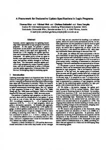


![NI USB-9219 User Guide and Specifications - National Instruments [PDF]](https://m.moam.info/img/260x300/ni-usb-9219-user-guide-and-specifications-national_648799ec098a9e846f8b45c3.jpg)


