A Deferrable Scheduling Algorithm for Real-Time Transactions

A Deferrable Scheduling Algorithm for Real-Time Transactions Maintaining Data Freshness Ming Xiong Bell Labs, Lucent Technologies [email protected]

Song Han City University of Hong Kong han [email protected]

Abstract

Kam-Yiu Lam City University of Hong Kong [email protected]

vironment. Each real-time data object is associated with a validity interval as the lifespan of the current data value defined based on the dynamic properties of the data object. A new data value needs to be installed into the database before the validity interval of its old value expires, i.e., the old one becomes temporally invalid. Otherwise, the RTDBS cannot detect and respond to environmental changes timely. In recent years, there has been tremendous amount of work devoted to this area [4, 9, 11, 12, 17, 18, 19, 21, 8, 22, 6]. To maintain temporal validity, sensor update transactions, which capture the latest status of the entities in the system environment, are generated to refresh the values of the real-time data objects periodically [17, 11, 22]. A sensor update transaction has an infinite number of periodic jobs, which have fixed length period and relative deadline. The update problem for periodic update transactions consists of two parts [22]: (1) the determination of the sampling periods and deadlines of update transactions; and (2) the scheduling of update transactions. Two methods have been proposed in prior work for minimizing the update workload while maintaining the data freshness. As explained in [17, 11], a simple method to maintain temporal validity of real-time data objects is to use the Half-Half (HH) scheme in which the update period for a real-time data object is set to be half of the validity interval length of the object. To further reduce the update workload, the More-Less (ML) scheme is proposed [22]. This paper presents our Deferrable Scheduling algorithm for Fixed Priority transactions (DS-FP) with the objective to minimize the update workload. We study the problem of data freshness maintenance for firm real-time update transactions in a single processor RTDBS. Distinct from the past work of HH and ML, which has a fixed period and relative deadline for each transaction, DS-FP adopts a sporadic task model. In contrast to ML in which a relative deadline is always equivalent to the worst-case response time of a transaction, DS-FP dynamically assigns relative deadlines to transaction jobs by deferring the sampling time of a transaction job as much as possible while still guaranteeing the temporal validity of real-time data to be updated. The deferral of a job’s sampling time results in a relative deadline

Periodic update transaction model has been used to maintain freshness (or temporal validity) of real-time data. Period and deadline assignment has been the main focus in the past studies such as the More-Less scheme [22] in which update transactions are guaranteed by the Deadline Monotonic scheduling algorithm [13] to complete by their deadlines. In this paper, we propose a novel algorithm, namely deferrable scheduling, for minimizing imposed workload while maintaining temporal validity of real-time data. In contrast to previous work, update transactions scheduled by the deferrable scheduling algorithm follow a sporadic task model. The deferrable scheduling algorithm exploits the semantics of temporal validity constraint of real-time data by judiciously deferring the sampling times of update transaction jobs as late as possible. We present a theoretical analysis of its processor utilization, which is verified in our experiments. Our experimental results also demonstrate that the deferrable scheduling algorithm is a very effective approach, and it significantly outperforms the MoreLess scheme in terms of reducing processor workload.

1 Introduction Real-time and embedded systems are used in many application domains that require timely processing of massive amount of real-time data. Examples of real-time data include sensor data in sensor networks, positions of aircrafts in an air traffic control system, and temperature as well as air pressure in an engine control environment. Such realtime data are typically stored in a real-time database system (RTDBS). They are used to model the current status of entities in a system environment. However, real-time data are different from traditional data stored in databases in that they have time semantics indicating that sampled values are valid only for a certain time interval [17, 15, 20]. The concept of temporal validity is first introduced in [17] to define the correctness of real-time data. A real-time data object is fresh (or temporally valid) if its value truly reflects the current status of the corresponding entity in the system en1

Proceedings of the Fourth International Workshop on Web Site Evolution (WSE’02) 0-7695-1804-4/02 $17.00 © 2002 IEEE

that is less than its worst-case response time, thus increases the separation of two consecutive jobs. This helps reducing processor workload produced by update transactions. The average processor utilization under DS-FP is theoretically analyzed. Our experimental study of DS-FP demonstrates that it is an effective algorithm for reducing the workload of real-time update transactions. It also verifies the accuracy of our theoretical estimation of average processor utilization under DS-FP. The rest of the paper is organized as follows: Section 2 reviews the existing approaches for freshness maintenance of real-time data. In Section 3, the Deferrable Scheduling algorithm for Fixed Priority transactions (DS-FP) is proposed and discussed in detail. Section 4 presents the performance studies and Section 5 briefly describes the related work. Finally, we conclude our study in Section 6.

Symbol

J

f r d

2 Background: Data Freshness Maintenance

Definition Real-time data object Update transaction updating The th job of Response time of J Computation time of transaction Validity (interval) length of Finishing time of J Release (Sampling) time of J Absolute deadline of J Period of transaction in ML Relative deadline of transaction in ML Separation of jobs (i.e., r r ) in DS-FP Relative deadline of J in DS-FP Average period of transaction in DS-FP Average relative deadline of transaction in DS-FP Average processor utilization in DS-FP

Table 1. Symbols and definitions.

Real-time data, whose state may become invalid with the passage of time, need to be refreshed by sensor update transactions generated by intelligent sensors that sample the value of real world entities. To monitor the states of entities faithfully, real-time data must be refreshed before they become invalid. The actual length of the temporal validity interval of a real-time data object is application dependent. For example, real-time data with validity interval requirements are discussed in [17, 18, 15]. One of the important design goals of RTDBSs is to guarantee that real-time data remain fresh, i.e., they are always valid.

are assumed to be kept in main memory. Associated with is a validity interval of length : transacupdates the corresponding data object tion . Because each update transaction updates the different data object, no concurrency control is considered for update transactions. We assume that a sensor always samples the value of a real-time data object at the beginning of its period, and the system is synchronous, i.e., all the first jobs of update transactions are initiated at the same time. For convenience, let d , f and r denote the absolute deadline, completion time, and sampling (release) time of the job J of , respectively. We also assume that jitter between sampling time and release time of a job is zero (readers are referred to [22] for how jitters can be handled). Formal definitions of the frequently used symbols are given in Table 1. Deadlines of update transactions are firm deadlines. The goal of Half-Half and More-Less, which adopt periodic and relative deadline task model, is to determine period so that all the update transactions are schedulable and CPU workload resulting from periodic update transactions is minimized. Both HH and ML assume a simple execution semantics for periodic transactions: a transaction must be executed once every period. However, there is no guarantee on when a job of a periodic transaction is actually executed within a period. Throughout this paper we assume the scheduling algorithms are preemptive and ignore all preemption overhead. For convenience, we use terms transaction and task interchangeably in this paper. Half-Half: In HH, the period and relative deadline of an update transaction are each typically set to be one-half of the data validity length [17, 11]. In Figure 1, the farthest distance of two consecutive jobs of (based on the sampling time r of job J and the deadline d of its next job) is . If , then the validity of real-time object is guaranteed as long as jobs of meet their deadlines. Un-

2.1 Temporal Validity for Data Freshness As real-time data values change continuously with time, depends on the the correctness of a real-time data object difference between the real-time status of the real world entity and the current sampling value of . Definition 2.1: A real-time data object (

) at time is temporally valid (or absolutely consistent) if its sampling time (r ) plus the validity interval ( ) of the data object is [17]. not less than , i.e., r A data value for real-time data object sampled at any time will be valid for following that up to . Next, we review existing approaches that adopt periodic task model for sensor update transactions.

2.2 Half-Half and More-Less In this section, traditional approaches for maintaining temporal validity, namely the Half-Half (HH) and MoreLess (ML) approaches are reviewed. refers to a set of periodic upIn this paper, and refers date transactions to a set of real-time data objects. All real-time data objects 2

Proceedings of the Fourth International Workshop on Web Site Evolution (WSE’02) 0-7695-1804-4/02 $17.00 © 2002 IEEE

Ji, j

Ji, j

T

J i, j+1

must be greater than or equal to , the worst-case execution time of , i.e., . Feasibility constraint: for a given set of update transactions, Deadline Monotonic scheduling algorithm [13] is used to schedule the transactions. Consequently, if has higher . priority than for

J i, j+1 T+2P i

T+P i

2Ci 2Pi

Figure 1. Extreme execution cases of jobs J J

and ML assigns priorities to transactions based on Shortest Validity First (SVF), i.e., in the inverse order of validity length and ties are resolved in favor of transactions with less slack for ). It assigns deadlines and periods to (i.e., as follows:

Pi+D i J i, ri,

j

J i,

j

di,

j

( =r i, j +D i )

ri,

j+1

( =r i, j+Pi )

f

j+1

di,

j+1

ri,

r

(1) (2)

j+2

( =r i, j+P i+Di ) ( =r i, j+2P i )

where f and r are finishing and sampling times of the first job of , respectively. Note that in a synchronous system, r and the first job’s response time is the worstcase response time in ML. In this paper, superscript ml is used to distinguish the finishing and sampling times in ML from those in DS-FP.

Figure 2. Illustration of More-Less scheme fortunately, this approach incurs unnecessarily high CPU workload of the update transaction in the RTDBSs compared to More-Less. More-Less: Consider the worst-case response time for any job of a periodic transaction where the response time is the difference between the transaction initiation time and the transaction completion time where is the offset within the period.

3 Deferrable Scheduling A scheduler is work-conserving if it never idles the processor while there is a job awaiting execution. All schedulers discussed in this paper are work-conserving. Next, we present our Deferrable Scheduling algorithm for Fixed Priority transactions (DS-FP), and compare it with ML.

Lemma 2.1: For a set of periodic transactions

3.1 Intuition of DS-FP

with transaction initiation time , the worst-case response time for any job of occurs for the first job of when . [13]

In ML, is determined by the first job’s response time, which is the worst-case response time of all jobs of . Thus, ML is pessimistic on the deadline and period assignment in the sense that it uses periodic task model that has a fixed period and deadline for each task, and the deadline is equivalent to the worst-case response time. It should be noted that the validity constraint can always be satisfied as . But processor workload is minimized long as . Otherwise, can always be increased only if to reduce processor workload as long as . Given release time r of job J and deadline d of job , J d r (3)

For , the transactions are synchronous. A time instant after which a transaction has the worst-case response time is called a critical instant, e.g., time is a critical instant for all the transactions if those transactions are synchronous. To minimize the update workload, ML is proposed to guarantee temporal validity [22], in which Deadline Monotonic (DM) [13] is used to schedule periodic update transactions. There are three constraints to follow for ( ):

guarantees that the validity constraint can be satisfied, as depicted in Figure 3. Correspondingly, the following equation follows directly from Eq. 3.

Validity constraint: the sum of the period and relative deadline of transaction is always less than or equal , as shown in Figure 2. to , i.e., Deadline constraint: the period of an update transaction is assigned to be more than half of the validity length of the object to be updated, while its corresponding relative deadline is less than half of the validity length of the same object. For to be schedulable,

r

r

d

r

(4)

If r is shifted onward to r along the time line in Figure 3, it does not violate Eq. 4. This shift can be achieved, e.g., in the ML schedule, if preemption to J from higher-priority transactions in r d is less 3

Proceedings of the Fourth International Workshop on Web Site Evolution (WSE’02) 0-7695-1804-4/02 $17.00 © 2002 IEEE

Note that schedule of all higher-priority jobs that are needs to be computed before released prior to d r d is computed. This computation can be invoked in a recursive process from jobs of lower-priority transactions to higher-priority transactions. Nevertheless, it does not require that schedule of all jobs should be constructed off-line before the task set is executed. Indeed, the computation of job deadlines and their corresponding release times is performed on-line while the transactions are being scheduled. We only need to compute the first jobs’ response times when system starts. Upon completion of job , is firstly derived from J , deadline of its next job, d Eq. 3, then the corresponding release time r is derived r d cannot be computed due from Eq. 5. If to incomplete schedule information of release times and absolute deadlines from higher-priority transactions, DS-FP computes their complete schedule information on-line until . Job J ’s it can gather enough information to derive r DS-FP scheduling information (e.g., release time, deadline, bookkeeping information, etc.) can be discarded after it completes and it is not needed by jobs of lower-priority transactions. This process is called garbage collection in DS-FP. Let J denote the set of jobs of all transactions whose deadlines have been computed by time . Also let denote the latest scheduled deadline of at , i.e., maximum of all d for jobs J of whose deadlines have been computed by ,

J i, j+1

Vi Ji, j

ri, j

Ji, j+1

d i, j

di, j+1

Vi d i, j+2

ri, j+1 Vi

d'i, j+2

r'i, j+1

Figure 3. Illustration of DS-FP scheduling (r is shifted to r )

than the worst-case preemption to the first job of . Thus, is temporal validity can still be guaranteed as long as J completed by its deadline d . The intuition of DS-FP is to defer the sampling time, , of J ’s subsequent job as late as possible while still r guaranteeing the validity constraint. Note that the sampling time of a job is also its release time, i.e., time that the job is ready to execute as we assume zero cost for sampling and no arrival jitter for a job for convenience of presentation. ’s release time reduces the relThe deferral of job J ative deadline of the job if its absolute deadline is fixed as is deferred to r in Figure in Eq. 3. For example, r in order 3, but it still has to complete by its deadline d to satisfy the validity constraint (Eq. 3). Thus its relative deadline, , becomes d r , which is less r . The deadline of J ’s subsequent than d , can be further deferred to r to satjob, J isfy the validity constraint. Consequently, the processor uti, and J lization for completion of three jobs, J , J then becomes . It is less than the utilizad r

J

d then the information of J

Definition 3.1: Let

denote the total cumulative processor demands made by all jobs of higher-priority transacduring time interval tion for from a schedule produced by a fixed priority scheduling algorithm. Then,

d

can be garbage collected.

tions whose parameters are shown in Table 2. The resulting periods and deadlines in HH and ML are shown in the and same table. Utilizations of HH and ML are , respectively. Figures 4 (a) and (b) depict the schedules produced by ML and DS-FP, respectively. It can be observed from both schedules that the release times of transaction jobs J , J , J , J are shifted from times in ML in DS-FP, respectively. to The DS-FP algorithm is described in Section 3.2.

Next, we discuss how much a job’s release time can be deferred. According to fixed priority scheduling theory, r can be derived backwards from its deadline d as follows: r

(7)

Example 3.1: Suppose that there are three update transac-

where is the total processor demands made by all . jobs of single transaction during

d

(6)

Given job J whose scheduling information has been computed at time , and , if

required for completion of the same tion d r amount of work in ML.

r

d J

3.2 Deferrable Scheduling Algorithm This section presents the DS-FP algorithm. It is a fixed priority scheduling algorithm. Given an update transaction has higher priority than if set , it is assumed that

(5) 4

Proceedings of the Fourth International Workshop on Web Site Evolution (WSE’02) 0-7695-1804-4/02 $17.00 © 2002 IEEE

T1

T2

T2 Release Time Shifting

T3

T3 Release Time Shifting

10 11 12 13

0

10

5

15

20

25

14

30

15

(a) Schedule with More-Less

16 17 18 19 0

10

5

15

20

25

30

20

(b) Schedule with DS-FP

21 22

Figure 4. Comparing ML and DS-FP schedules

23 25 26

Half-Half

27 28

1 2 3

1 2 2

5 10 20

0.2 0.2 0.1

4 7 14

1 3 6

2.5 5 10

29 30

Table 2. Parameters and results for Example 3.1 . Transaction priority assignment policy in DS-FP is the same as in ML, i.e., Shortest Validity First. Algorithm 3.1 presents the DS-FP algorithm. For convenience of presentation, garbage collection is omitted in the algorithm. There are two cases for the DS-FP algorithm: 1) At system initialization time, Lines 13 to 20 iteratively calculate the first job’s response time for . The first job’s deadline is set as its response time (Line 21). 2) Upon completion of ’s job J , the deadline of its next job (J ), d , is derived at Line 27 so that the far’s finishing thest distance of J ’s sampling time and J time is bounded by the validity length (Eq. 3). Then the sampling time of J ,r , is derived backwards from its deadline by accounting for the interference from higherpriority transactions (Line 29).

Algorithm 3.2 ScheduleRT( , , Input: J with Output: r .

1 2 3 4 5 6 7 8 9 10 11

Algorithm 3.1 DS-FP algorithm: Input: A set of update transactions with known and . Output: Construct a partial schedule if otherwise, reject.

1 2 3

//

system initialization time // Initialization – Latest Scheduled Deadline of

12 13

’s jobs.

5

7 8 9

and d

,d

):

.

oldHPPreempt // initial HP preemptions hpPreempt r d // Calculate HP preemptions backwards from d . hpPreempt CalcHPPreempt r d while hpPreempt oldHPPreempt do // Accounting for the interference of HP tasks r d hpPreempt if r d then abort endif oldHPPreempt hpPreempt hpPreempt GetHPPreempt r d end return r

Function ScheduleRT d (Algorithm 3.2) calculates the release time r with known computation time and deadline d . It starts with release time r d , then iteratively calculates r d , the total cumulative processor demands made by all higher-priority jobs of J during interval r d , and adjusts r by accounting for interference from higher-priority transactions (Lines 5 to 12). The computation of r continues until interference from higher-priority transactions does not change in an iteration. In particular, Line 9 detects an infeasible schedule. A schedule becomes infeasible under DS-FP if d , i.e., release time of J becomes earr lier than the deadline of its preceding job J . Function

is feasible;

4

6

f // Calculate higher-priority (HP) preemptions. oldHPPreempt // initial HP preemptions hpPreempt CalcHPPreempt f while hpPreempt oldHPPreempt do // Accounting for the interference of HP tasks f r hpPreempt if f then abort endif oldHPPreempt hpPreempt hpPreempt CalcHPPreempt f end d f end return upon completion of J // Schedule release time for J . d r // get next deadline for J // r is also the sampling time for J r ScheduleRT d return

// is the latest scheduled job of for to do // Schedule finish time for . r 5

Proceedings of the Fourth International Workshop on Web Site Evolution (WSE’02) 0-7695-1804-4/02 $17.00 © 2002 IEEE

GetHPPreempt scans interval , adds up total preemptions from , and returns , the cumulative processor demands of during from schedule that has been built.

Job

Algorithm 3.3 CalcHPPreempt( , , , ): Input: J , and a time interval . Output: Total cumulative processor demands from higher-priority transactions during . // Record latest scheduled job of

1 2

.

d if

5

then // No preemptions from higher-priority tasks. return 0 elsif then // Get preemptions from // because ’s schedule is complete before . return GetHPPreempt endif // build up to or exceeding for . for to do while d do d r r d

6 7 8 9 10 11 12 13 14 15 16

19 20 21

Function CalcHPPreempt (Algorithm 3.3) , the total cumulative processor decalculates mands made by all higher-priority jobs of J during interval . Line 7 indicates that , ’s schedule is completely built before time . This is because ’s schedule cannot be completely built before unless schedules of its higher-priority transactions are complete before . In this case, the function simply returns amount of higher-priority preemptions for during by invoking GetHPPreempt , which returns . If any higher-priority transaction does not have a complete schedule during , its schedule up to or exceeding is built on the fly (Lines 14 to 19). This enables the computation of . The latest scheduled , indicates the latest deadline of deadline of ’s job, ’s jobs that have been computed. The worst-case complexity of ScheduleRT is assuming that is a constant. The following lemma states an important property of ScheduleRT when it terminates. Lemma 3.1: Given a synchronous update transaction set

d

ML (0, 6) (14, 20) (28, 34) ...

DS-FP (0, 6) (18, 20) (35, 38) ...

Example 3.2: Table 3 presents comparison of (release time, deadline) pairs of , and jobs before time in Example 3.1, which are assigned by ML and DS-FP (Algorithm 3.1). Note that has same release times and deadlines for all jobs under ML and DS-FP. However, J , J , J , J , and J have different release times and deadlines under ML and DS-FP. Algorithm 3.1 starts at system initialization time. It calculates deadlines for J , J , J . Upon completion of J at time 6, d is set to r + . Then Algorthim 3.1 invokes ScheduleRT at Line 29, which will derive r . At this moment, Algorithm 3.1 has already calculated the complete schedule up to d (time ). But the schedule in the interval has only been partially derived. Specifically, only schedule information of J , J , J , J J , and J has been derived for and . Algorithm 3.2 (ScheduleRT) obtains r at Line 3, then invokes CalcHPPreempt . Algorithm 3.3 (CalcHPPreempt) finds out that , then it jumps to the loop starting at Line 13 to build the complete schedule of and in the interval , where the release times and deadlines for J , J , J , J , and J are derived. Thus, higher-priority transactions and have a complete schedule before time . Note that r and d for J are derived when we calculate r and d such that the complete schedule up to d has been built for transactions with priority higher than . by earlier calculation, d is set to . As r is set to It derives r backwards from d and sets it to because . Similarly, d and r are set to and , respectively.

d end end return GetHPPreempt

and ScheduleRT

DS-FP (0, 3) (7, 10) (14, 17) (22, 24) (30, 32) (38, 40) ...

Proof: This can be proved by contradiction. Suppose that when ScheduleRT d terminates at . Let at at the same Line 14 in CalcHPPreempt. As line, ScheduleRT has not reached the point to terminte. This contradicts the assumption. The next example illustrates how DS-FP algorithm works with the transaction set in Example 3.1.

17 18

ML (0, 3) (7, 10) (14, 17) (21, 24) (28, 31) (35, 38) ...

Table 3. Release time and deadline comparison holds when Schedd terminates at time . uleRT

3 4

ML/DS-FP (0,1) (4,5) (8,9) (12,13) (16,17) (20,21) (24,25) (28,29) (32,33) (36,37)

, 6

Proceedings of the Fourth International Workshop on Web Site Evolution (WSE’02) 0-7695-1804-4/02 $17.00 © 2002 IEEE

3.3 Comparison of DS-FP and ML

Therefore,

Note that ML is based on the periodic task model, while DS-FP adopts one similar to the sporadic task model [1]. However, the relative deadline of a transaction in DS-FP is not fixed. Theoretically, the separation of two consecutive jobs of in DS-FP satisfies the following condition: WCRT

(13) Given arbitrarily large holds:

, the following equation

(8)

(14)

where WCRT is the worst-case response time of jobs of in DS-FP. Note that the maximal separation of J and , , cannot exceed J , which can be obtained when there are no higher-priority preemptions for the execution of job J (e.g., the highest priority transaction always has separation for J and J ). Thus, the processor utilization for DS, which is the CPU FP should be greater than workload resulting from the maximal separation of each transaction. ML can be regarded as a special case of DS-FP in which and deadline d sampling (or release) time r can be specified as follows:

and can Following Eq. 11 and 14, be calculated (from the highest priority transaction to the lowest priority transaction ) as following, respectively:

d

r

r

d

(15) (16) Finally, , the average utilization of the transaction set under DS-FP can be estimated as: (17)

(9) r

It is clear that r in ML.

f

f f

The following example illustrates how the average utilization is estimated.

(10) when r

Example 3.3: Given the transaction set in Table 2, we cal-

culate the average relative deadline and period of as follows:

3.4 Theoretical Analysis of DS-FP Utilization Given a transaction set that can be scheduled by ML, we now present the analysis of average processor utilization , let denote the averof DS-FP. Suppose age processor utilization under DS-FP. We have the average relative deadline of , namely , as follows:

where denotes the average number of times that higher priority transaction occurs during an interval of length . Therefore, represents the average and response time of . It is obvious that for any , where is the average period for . Thus,

The average processor utilization is . Given the transaction set in Table 2, it can be verified that the processor utilization for the first time units is , which is very close to our theoretical estimation and lower than the processor utilization from ML ( ).

4 Performance Evaluation (11) Let and r and d

r

This section presents important results from our experimental studies of the proposed deferrable scheduling algorithm (DS-FP). We compare DS-FP with the More-Less (ML) algorithm, which outperforms Half-Half [22].

denote r in Eq. 4, respectively. It follows that (12)

Given the first

jobs of

4.1 Simulation Model and Parameters

, we have

We have conducted two sets of experiments comparing the performance of DS-FP and ML. In the first set of experiments, we compare the update transaction workloads produced by DS-FP and ML. It is demonstrated that DS-FP 7

Proceedings of the Fourth International Workshop on Web Site Evolution (WSE’02) 0-7695-1804-4/02 $17.00 © 2002 IEEE

Parameter Class

Parameters

System Update Transactions Triggered Transactions

Length CPU Time Length Arrival Rate Slack Factor

Meaning No. of CPU No. of real-time data objects Validity interval of CPU time for updating No. of data to update CPU time per data access No. of data to access Transaction triggering rate Transaction slack factor

Table 4. Experimental parameters Figure 5. CPU workloads comparison Parameter Class

Parameters

System Update Transactions Triggered Transactions

Length CPU Time (ms) Length Arrival Rate Slack Factor

Meaning 1 [50, 300] [4000, 8000] [5, 15] 1 [3, 5] [5, 15] [5, 10] 8

in experiments are presented in Tables 4 and 5. The baseline values for the parameters follow those used in [22], which are originally from air traffic control applications. Three classes of parameters are defined: system parameters, update transaction parameters and triggered transaction parameters. For system configurations, we only consider a single CPU, main memory based RTDBS. The number of real-time data objects is varied from 50 to 300 and it is assumed that the validity interval length of each real-time data object is uniformly varied from 4000 to 8000 ms. For update transactions, it is assumed that each transaction updates one real-time data object, and the CPU time for each transaction is uniformly varied from 5 to 15 ms. For the triggered transactions, we assume that the number of realtime data objects accessed by each transaction is uniformly varied from 5 to 15, while accessing each data object takes 3 to 5 ms of CPU time. The inter-arrival time of the triggered transactions follows exponential distribution and the arrival rate is varied from 5 to 10 transactions per second. The slack factor determines the slack of a transaction before , its deadline expires and it is fixed at 8. Let and denote the arrival time, total execution time and deadline of triggered transaction , the deadline of can be calculated as follows in our experiments: Slack Factor

Table 5. Experimental settings produces lower CPU workload than ML. Also, we demonstrate that the increase of average sampling period from DSFP is the main reason for its lower workload. In the second set of experiments, we study the performance of DS-FP and ML under mixed transaction workloads: a class of update transactions that maintain the freshness (validity) of realtime data objects, and a class of triggered transactions that are triggered by the changes of real-time data values. The triggered transactions need to read a group of real-time data objects for decision making. Given transactions belonging to different classes, update transactions are assigned higher priorities than the triggered transactions. For simplicity of the simulation study, only one version of a real-time data object is maintained. Upon refreshing a real-time data object, the older version is discarded. The primary performance metrics used in the experiments are CPU workload, mean transaction response time and missed deadline ratio (MDR) of the triggered transactions. We also measure the age of data (AGE) that indicates how old the real-time data object is at the commit time of a triggered transaction. Suppose that the current data value for real-time data object is sampled at time , and its data value is valid until . If a triggered transaction that reads the value of commits at time , its AGE is defined as:

In the experiments, percent confidence intervals have been obtained whose widths are less than percent of the point estimate for the performance metrics.

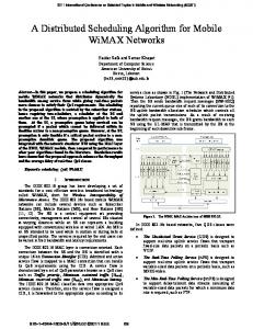
4.2 Expt. 1: Comparison of CPU Workloads In this set of experiments, the CPU workloads of update transactions produced by ML and DS-FP are quantitatively compared. Update transactions are generated randomly according to the parameter settings in Table 5. The resulting CPU workloads generated from ML and DS-FP are depicted in Figure 5. From the results, we observe that DS-FP’s CPU workload is consistently lower than that of ML. In fact, the difference widens as the number of update transactions increases. The difference reaches

A summary of the parameters and default settings used 8

Proceedings of the Fourth International Workshop on Web Site Evolution (WSE’02) 0-7695-1804-4/02 $17.00 © 2002 IEEE

Figure 6. Average sampling period comparison

Figure 7. Response time comparison

when the number of transactions is 300. It is also observed that our experimental results of DS-FP match the average CPU workload calculated from the theoretical estimation (Eq. 17). Last but not least, the DS-FP CPU workload is , which is the CPU only slightly higher than workload resulting from the maximal separation of each transaction (see Section 3.3). In fact, the difference is insignificant in Figure 5. The improvement of CPU workload under DS-FP is due to the fact that DSFP adaptively samples real-time data objects at a lower rate. This is verified by the average sampling periods of update transactions obtained from experiments. Figure 6 shows the average sampling period for each transaction in DS-FP . Given a set when the number of update transactions is of update transactions, the period of transaction in ML ( ) is a constant and it can be calculated off-line [22], while the separation of sampling times of two consecutive jobs from the same transaction in DS-FP is dynamic and it is obtained on-line in the experiments. The mean value of , for the separations, i.e., the average sampling period, transaction is calculated as follows, where is the number of jobs generated by in the experiments.

4.3 Expt. 2: Co-scheduling of Mixed Workloads In this set of experiments, performances of mixed transactions are compared for ML and DS-FP in two scenarios: 1) Triggered transactions do not have deadlines. Their average response time and age of data at commit time are compared for ML and DS-FP; 2) Triggered transactions have deadlines. Their missed deadline ratios (MDRs) are compared for ML and DS-FP. In both cases, update transactions are scheduled by either ML or DS-FP for comparison. The parameter settings in the experiments are listed in Table 5. 4.3.1 Comparison of Average Response Time In these experiments, triggered transactions do not have deadlines. We fix the triggered transactions’ arrival rate at 10 transactions per second and the CPU time for accessing each real-time data object at 3 ms. We vary the number of update transactions from 50 to 250 in order to show its impact on the performance of average response times of the triggered transactions. We also consider two cases: 1) Triggered transactions obey data-deadline [21], which means that triggered transactions are aborted and restarted if the value of a real-time data object accessed by the transaction expires before the transaction commits; 2) Triggered transactions do not obey data-deadline, which means that the triggered transactions can still commit if the values of its accessed real-time data objects expire. Informally, datadeadline is a deadline assigned to a transaction due to the temporal constraints (i.e., validity interval length) of the data accessed by the transaction. For details of the concept of data-deadline, readers are referred to [21]. In Figure 7, the average response time of triggered transactions with update transactions scheduled by DS-FP is consistently lower than that of triggered transactions with update transactions scheduled by ML. For example, there is improvement in the response time of triggered transa actions if the number of update transactions is no matter whether data-deadline is obeyed or not. Figure 7 also demonstrates that the average response time of the triggered transactions in ML increases dramatically when the number

(18)

is consistently larger In Figure 6, it is observed that while the difference ( ) increases with than the decrease of the transaction’s priority. DS-FP reduces the average sampling rate more for lower-priority transactions, thus greatly reduces the workload of CPU. Figure 6 ) increases similarly also demonstrates that the trend of ( although it fluctuates. In summary, when a set of update transactions is scheduled by DS-FP to maintain temporal validity of real-time data objects, it produces a schedule with a much lower CPU workload than ML. Thus more CPU capacity is available for other transactions, e.g., triggered transactions. 9

Proceedings of the Fourth International Workshop on Web Site Evolution (WSE’02) 0-7695-1804-4/02 $17.00 © 2002 IEEE

Figure 8. Average age of data

Figure 9. Missed deadline ratio comparison

. This is because the CPU of update transactions reaches is almost saturated by the workload generated from update transactions in the ML case if the number of update trans. However, the CPU workload of update actions reaches transactions generated from DS-FP is much lower than that from ML.

served that the difference of MDRs of triggered transactions widens as the number of update transactions increases. In summary, DS-FP also provides better performance in the co-scheduling of mixed workloads where transactions can be triggered by the changes of values of real-time data objects. It greatly improves the average transaction response time and missed deadline ratio while only increases the average age of data insignificantly.

4.3.2 Comparison of Average Age of Data In these experiments, triggered transactions again do not have deadlines, and data-deadline is not obeyed by the triggered transactions. We compare the average age of data (AGE) accessed by the triggered transactions for ML and DS-FP at transaction commit time. Because DS-FP samples the data at lower rate, it is unclear how much impact the lower sampling rate has on the age of data at the commit time of a triggered transaction. Figure 8 demonstrates that DS-FP’s average age of data at commit time of the triggered transactions is only slightly larger than that of ML. In fact, the difference is very small and it can be totally ignored.

5 Related Work There has been a lot of work on RTDBSs in which validity intervals are associated with real-time data [19, 9, 10, 11, 4, 21, 8, 12, 6, 5, 22]. [6] presents a vehicular application with embedded engine control systems, and an on-demand scheduling algorithm for enforcing base and derived data freshness. [5] proposes an algorithm (ODTB) for updating data items that can skip unnecessary updates allowing for better utilization of the CPU in the vehicular application. In [11], similarity-based principles are coupled with the Half-Half approach to adjust real-time transaction load by skipping the execution of task instances. The concept of data-deadline is proposed in [21]. It also proposes datadeadline based scheduling, forced-wait and similarity-based scheduling techniques to maintain the temporal validity of real-time data and meet transaction deadlines in RTDBSs. Our work is related to the More-Less scheme in [22, 12]. More-Less guarantees a bound on the sampling time of a periodic transaction job and the finishing time of its next job. But, as we showed, the deadline and period of a periodic transaction are derived from the worst-case response time of the transaction. This is different from sporadic task model based DS-FP algorithm in which deadline of a transaction job is derived adaptively, and the separation of two consecutive jobs is not a constant. DS-FP reduces CPU workload resulting from update transactions further by adaptively adjusting the separation of two consecutive jobs while satisfying the validity constraint. DS-FP is also different from the distance constrained scheduling, which guarantees a bound of the finishing times of two consecutive instances of a task

4.3.3 Comparison of Missed Deadline Ratio (MDR) Different from previous experiments, in this set of experiments we suppose that the triggered transactions have deadlines and they obey the data-deadline constraint. A triggered transaction that cannot commit before the validity of its accessed data expires has to be aborted, and restarted later if it has not missed its deadline. In such a case, a data-deadline is imposed on the triggered transaction due to the temporal constraints resulting from data validities. The triggered transactions are scheduled by the earliest deadline first (EDF) scheduling algorithm [14]. The CPU time for accessing a real-time data object is fixed at 5 ms. Figure 9 shows that the MDR of the triggered transactions under DSFP is much lower than that under ML. For example, when and the triggered the number of update transactions is triggered transtransactions are scheduled by EDF, only actions miss their deadlines under DS-FP, but around triggered transactions miss their deadlines under ML. This is because the CPU workload of update transactions under ML is much higher than that under DS-FP. It can be ob10

Proceedings of the Fourth International Workshop on Web Site Evolution (WSE’02) 0-7695-1804-4/02 $17.00 © 2002 IEEE

[7]. The EDL algorithm proposed in [3] processes tasks as late as possible based on the Earliest Deadline scheduling algorithm [14]. EDL assumes that all deadlines of tasks are given whereas DS-FP derives deadlines dynamically. Finally, our DS-FP algorithm is applicable to the scheduling of age constraint tasks in real-time systems [2, 16] to reduce processor utilization.

[5] T. Gustafsson, J. Hansson, “Data Management in Real-Time Systems: a Case of On-Demand Updates in Vehicle Control Systems,” IEEE Real-Time and Embedded Technology and Applications Symposium, pp. 182-191, 2004. [6] T. Gustafsson and J. Hansson, “Dynamic on-demand updating of data in real-time database systems,” ACM SAC, 2004. [7] C. C. Han, K. J. Lin and J. W.-S. Liu, “Scheduling Jobs with Temporal Distance Constraints,” SIAM Journal of Computing, Vol. 24, No. 5, pp. 1104 - 1121, October 1995. [8] K. D. Kang, S. Son, J. A. Stankovic, and T. Abdelzaher, “A QoS-Sensitive Approach for Timeliness and Freshness Guarantees in Real-Time Databases,” EuroMicro Real-Time Systems Conference, June 2002. [9] T. Kuo and A. K. Mok, “Real-Time Data Semantics and Similarity-Based Concurrency Control,” IEEE Real-Time Systems Symposium, December 1992. [10] T. Kuo and A. K. Mok, “SSP: a Semantics-Based Protocol for Real-Time Data Access,” IEEE Real-Time Systems Symposium, December 1993. [11] S. Ho, T. Kuo, and A. K. Mok, “Similarity-Based Load Adjustment for Real-Time Data-Intensive Applications,” IEEE Real-Time Systems Symposium, 1997. [12] K.Y. Lam, M. Xiong, B. Liang and Y. Guo, “Statistical Quality of Service Guarantee for Temporal Consistency of Realtime Data Objects”, IEEE Real-Time Systems Symposium, 2004. [13] J. Leung and J. Whitehead, “On the Complexity of FixedPriority Scheduling of Periodic Real-Time Tasks,” Performance Evaluation, 2(1982), 237-250. [14] C. L. Liu, and J. Layland, “Scheduling Algorithms for Multiprogramming in a Hard Real-Time Environment,” Journal of the ACM, 20(1), 1973. [15] D. Locke, “Real-Time Databases: Real-World Requirements,” in Real-Time Database Systems: Issues and Applications, edited by Azer Bestavros, Kwei-Jay Lin and Sang H. Son, Kluwer Academic Publishers, pp. 83-91, 1997. [16] L. Lundberg, “Utilization Based Schedulability Bounds for Age Constraint Process Sets in Real-Time Systems,” RealTime Systems, 23(3), pp. 273-295, 2002. [17] K. Ramamritham, “Real-Time Databases,” Distributed and Parallel Databases 1(1993), pp. 199-226, 1993. [18] K. Ramamritham, “Where Do Time Constraints Come From and Where Do They Go ?” International Journal of Database Management, Vol. 7, No. 2, Spring 1996, pp. 4-10. [19] X. Song and J. W. S. Liu, “Maintaining Temporal Consistency: Pessimistic vs. Optimistic Concurrency Control,” IEEE Transactions on Knowledge and Data Engineering, Vol. 7, No. 5, pp. 786-796, October 1995. [20] J. A. Stankovic, S. Son, and J. Hansson, “Misconceptions About Real-Time Databases,” IEEE Computer, Vol. 32, No. 6, pp. 29-36, June 1999. [21] M. Xiong, K. Ramamritham, J. A. Stankovic, D. Towsley, and R. M. Sivasankaran, “Scheduling Transactions with Temporal Constraints: Exploiting Data Semantics,” IEEE Transactions on Knowledge and Data Engineering, 14(5), 1155-1166, 2002. [22] M. Xiong and K. Ramamritham, “Deriving Deadlines and Periods for Real-Time Update Transactions,” IEEE Transactions on Computers, 53(5), pp. 567-583, 2004.

6 Conclusions and Future Work This paper proposed a novel algorithm – deferrable scheduling for fixed priority transactions (DS-FP). Distinct from past studies of maintaining freshness (or temporal validity) of data in which the periodic task model is adopted, DS-FP adopts the sporadic task model. The deadlines of jobs and separation of two consecutive jobs of an update transaction are adjusted judiciously so that the farthest distance of the sampling time of a job and the completion time of its next job is bounded by the validity length of the updated real-time data. We proposed a theoretical estimation of the processor utilization of DS-FP, which is verified in our experimental studies. It is also demonstrated in our experiments that DS-FP greatly reduces processor workload compared to ML. Thus, DS-FP can improve the performance of triggered transactions when it is used by a RTDBS to track environmental changes. We intend to investigate the feasibility of DS-FP in our future work. For example, it is neither clear what a sufficient and necessary condition is for feasibility of DS-FP, nor is it clear how much DS-FP can improve the feasibility of update transactions compared to ML. Moreover, the concept of deferrable scheduling is only used to schedule update transactions with fixed priority in this paper. It is possible for the same concept to be used in the scheduling of update transactions with dynamic priority, e.g., in the Earliest Deadline scheduling [14, 3] of update transactions.

Acknowledgement This work was partially supported by the Research Grants Council of the Hong Kong Special Administrative Region, China [Project No. CityU 1076/02E].

References [1] S. K. Baruah, A. K. Mok, L. E. Rosier, “Preemptively Scheduling Hard-Real-Time Sporadic Tasks on One Processor,” IEEE Real-Time Systems Symposium, December 1990. [2] A. Burns and R. Davis, “Choosing task periods to minimise system utilisation in time triggered systems,” in Information Processing Letters, 58 (1996), pp. 223-229. [3] H. Chetto and M. Chetto, “Some Results of the Earliest Deadline Scheduling Algorithm,” IEEE Transactions on Software Engineering, Vol. 15, No. 10, pp. 1261-1269, October 1989. [4] R. Gerber, S. Hong and M. Saksena, “Guaranteeing Endto-End Timing Constraints by Calibrating Intermediate Processes,” IEEE Real-Time Systems Symposium, December 1994.

11

Proceedings of the Fourth International Workshop on Web Site Evolution (WSE’02) 0-7695-1804-4/02 $17.00 © 2002 IEEE